When I started work at Brilliant a couple of weeks ago, I learned that one of my new colleagues, Michelle McSweeney, just published a book called OK, which is all about the word OK.
As we discussed the joys and miseries of publishing, Michelle mentioned that she had found a typo in the book after publication. So naturally I took it as a challenge to find the typo. While I was searching, I enjoyed the book very much. If you are interested in etymology, linguistics, and history, I recommend it!
As it turned out, I found exactly one typo. When I told Michelle, she asked me nervously which page it was on. Page 17. She looked disappointed – that was not the same typo she found.
Now, for people who like Bayesian statistics, this scenario raises some questions:
After our conversation, how many additional typos should we expect there to be?
If she and I had found the same typo, instead of different ones, how many typos would we expect?
As it happens, I used a similar scenario as an example in Think Bayes. So I was able to reuse some code and answer these questions.
It’s been a while since anyone said “killer app” without irony, so let me remind you that a killer app is software “so necessary or desirable that it proves the core value of some larger technology,” quoth Wikipedia. For example, most people didn’t have much use for the internet until the world wide web was populated with useful content and the first generation of browsers made it easy to access.
So what is the Bayesian killer app? That is, for people who don’t know much about Bayesian methods, what’s the application that demonstrates their core value? I have a nomination: Thompson sampling, also known as the Bayesian bandit strategy, which is the foundation of Bayesian A/B testing.
I’ve been writing and teaching about Bayesian methods for a while, and Thompson sampling is the destination that provides the shortest path from Bayes’s Theorem to a practical, useful method that is meaningfully better than the more familiar alternative, hypothesis testing in general and Student’s t test in particular.
So what does that path look like? Well, funny you should ask, because I presented my answer last November as a tutorial at PyData Global 2022, and the video has just been posted:
This tutorial is a hands-on introduction to Bayesian Decision Analysis (BDA), which is a framework for using probability to guide decision-making under uncertainty. I start with Bayes’s Theorem, which is the foundation of Bayesian statistics, and work toward the Bayesian bandit strategy, which is used for A/B testing, medical tests, and related applications. For each step, I provide a Jupyter notebook where you can run Python code and work on exercises. In addition to the bandit strategy, I summarize two other applications of BDA, optimal bidding and deriving a decision rule. Finally, I suggest resources you can use to learn more.
Outline
Problem statement: A/B testing, medical tests, and the Bayesian bandit problem
Prerequisites and goals
Bayes’s theorem and the five urn problem
Using Pandas to represent a PMF
Estimating proportions
From belief to strategy
Implementing and testing Thompson sampling
More generally: two other examples of BDA
Resources and next steps
Prerequisites
For this tutorial, you should be familiar with Python at an intermediate level. We’ll use NumPy, SciPy, and Pandas, but I’ll explain what you need to know as we go. You should be familiar with basic probability, but you don’t need to know anything about Bayesian statistics. I provide Jupyter notebooks that run on Colab, so you don’t have to install anything or prepare ahead of time. But you should be familiar with Jupyter notebooks.
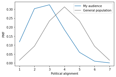
My audience skews left; that is, the people who read my blog are more liberal, on average, than the general population. For example, if I surveyed my readers and asked where they place themselves on a scale from liberal to conservative, the results might look like this:
To be clear, I have not done a survey and this is fake data, but if it were real, we would conclude that my audience is more liberal, on average, than the general population. So in the normal use of the word skew, we might say that this distribution “skews to the left”.
But according to statisticians, that would be wrong, because within the field of statistics, skew has been given a technical meaning that is contrary to its normal use. Here’s how Wikipedia explains the technical definition:
positive skew: The right tail is longer; the mass of the distribution is concentrated on the left of the figure. The distribution is said to be right-skewed, right-tailed, or skewed to the right, despite the fact that the curve itself appears to be skewed or leaning to the left; right instead refers to the right tail being drawn out and, often, the mean being skewed to the right of a typical center of the data. A right-skewed distribution usually appears as a left-leaning curve.
https://en.wikipedia.org/wiki/Skewness
By this definition, we would say that the distribution of political alignment in my audience is “skewed to the right”. It is regrettable that the term was defined this way, because it’s very confusing.
Recently I ran a Twitter poll to see what people think skew means. Here are the results:
Interpreting these results is almost paradoxical: the first two responses are almost equally common, which proves that the third response is correct. If the statistically-literate people who follow me on Twitter don’t agree about what skew means, we have to treat it as ambiguous unless specified.
The comments suggest I’m not the only one who thinks the technical definition is contrary to intuition.
This has always been confusing for me, since the shape of a right-skewed distribution looks like it’s “leaning” to the left…
I learnt it as B, but there’s always this moment when I consciously have to avoid thinking it’s A.
This is one of those things where once I learned B was right, I hated it so much that I never forgot it.
It gets worse
If you think the definition of skew is bad, let’s talk about bias. In the context of statistics, bias is “a systematic tendency which causes differences between results and fact”. In particular, sampling bias is bias caused by a non-representative sampling process.
In my imaginary survey, the mean of the sample is less than the actual mean in the population, so we could say that my sample is biased to the left. Which means that the distribution is technically biased to the left and skewed to the right. Which is particularly confusing because in natural use, bias and skew mean the same thing.
So 20th century statisticians took two English words that are (nearly) synonyms, and gave them technical definitions that can be polar opposites. The result is 100 years of confusion.
For early statisticians, it seems like creating confusing vocabulary was a hobby. In addition to bias and skew, here’s a partial list of English words that are either synonyms or closely related, which have been given technical meanings that are opposites or subtly different.
accuracy and precision
probability and likelihood
efficacy and effectiveness
sensitivity and specificity
confidence and credibility
And don’t get me started on “significance”.
If you got this far, it seems like you are part of my audience, so if you want to answer a one-question survey about your political alignment, follow this link. Thank you!
My poll and this article were prompted by this excellent video about the Central Limit Theorem:
Around the 7:52 mark, a distribution that leans left is described as “skewed towards the left”. In statistics jargon, that’s technically incorrect, but in this context I think it’s is likely to be understood as intended.