July 2019 – Probably Overthinking It

Left, right, part 2

July 27, 2019 AllenDowney

In the previous article, I looked at data from the General Social Survey (GSS) to see how political alignment in the U.S. has changed, on the axis from conservative to liberal, over the last 50 years.

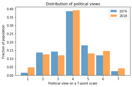
The GSS asks respondents where they place themselves on a 7-point scale from “extremely liberal” (1) to “extremely conservative” (7), with “moderate” in the middle (4).

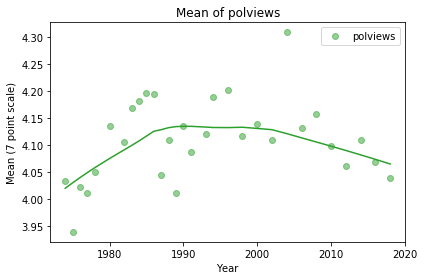
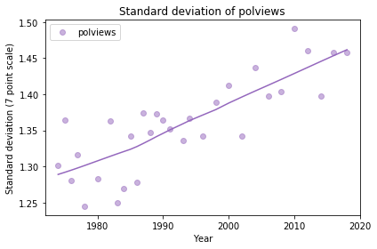
In the previous article I computed the mean and standard deviation of the responses as a way of quantifying the center and spread of the distribution. But it can be misleading to treat categorical responses as if they were numerical. So let’s see what we can do with the categories.

The following plot shows the fraction of respondents who place themselves in each category, plotted over time:

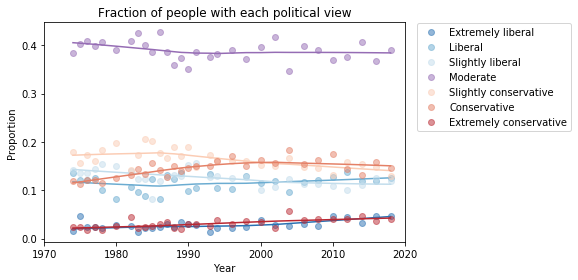
My initial reaction is that these lines are mostly flat. If political alignment is changing in the U.S., it is changing slowly, and the changes might not matter much in practice.

If we look more closely, it seems like the number of people who consider themselves “extreme” is increasing, and the number of moderates might be decreasing. The following plot shows a closer look at the extremes.

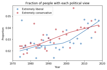
There is some evidence of polarization here, but we should not make too much of it. People who consider themselves extreme are still less than 10% of the population, and moderates are still the biggest group, at almost 40%.

To get a better sense of what’s happening with the other groups, I reduced the number of categories to 3: “Conservative” at any level, “Liberal” at any level, and “Moderate”. Here’s what the plot looks like with these categories:

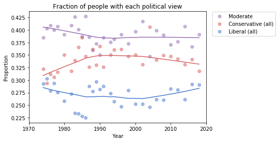
Moderates make up a plurality; conservatives are the next biggest group, followed by liberals.

From 1974 to 1990, the number of people who call themselves “Conservative” was increasing, but it has decreased ever since. And the number of “Liberals” has been increasing since 2000.

At least, that’s what this plot seems to show. We should be careful about over-interpreting patterns that might be random noise. And we might not want to take these categories too seriously, either.

The hazards of self-reporting

There are several problems with self-reported labels like this.

First, political beliefs are multi-dimensional. “Conservative” and “liberal” are labels for collections of ideas that sometimes go together. But most people hold a mixture of these beliefs.

Also, these labels are relative; that is, when someone says they are conservative, what they often mean is that they are more conservative than the center of the population, or where they think the center is, for the population they have in mind.

Finally, nearly all survey responses are subject to social desirability bias, which is the tendency of people to give answers that make them look better or feel better about themselves.

Over time, the changes we see in these responses depend on actual changes in political beliefs, but they also depend on where the center of the population is, where people think the center is, and the perceived desirability of the labels “liberal”, “conservative”, and “moderate”.

So, in the next article we’ll look more closely at changes in beliefs and attitudes, not just labels.

I am planning to turn these articles into a case study for an upcoming Data Science class, so I welcome comments and questions.

The code I used to generate these figures is in this Jupyter notebook.

Right, left, apart, together?

July 26, 2019 AllenDowney

Is the United States getting more conservative? With the rise of the alt-right, Republican control of Congress, and the election of Donald Trump, it might seem so.

Or is the country getting more liberal? With the 2015 Supreme Court decision supporting same-sex marriage, the incremental legalization of marijuana, and recent proposals to expand public health care, you might think so.

Or maybe the country is becoming more polarized, with moderates choosing sides and partisans moving to the extremes.

In a series of articles, I’ll use data from the General Social Survey (GSS) to explore these questions. The GSS goes back to 1972; every second year they survey a representative sample of U.S. residents and ask questions about their political beliefs. Many of the questions have been unchanged for almost 50 years, making it possible to observe long-term trends.

In this article, I’ll look at political alignment, that is, whether the respondents consider themselves liberal or conservative. In subsequent articles, I’ll explore their political beliefs on a range of topics.

Political alignment

From 1974 to the most recent cycle in 2018, the GSS asked the following question, “We hear a lot of talk these days about liberals and conservatives.
I’m going to show you a seven-point scale on which the political views that people might hold are arranged from extremely liberal–point 1–to extremely conservative–point 7. Where would you place yourself on this scale?”

The following figure shows the distribution of responses in 1974 and 2018.

In 2018, it looks like there are more 1s (Extremely Liberal) and maybe more 7s (Extremely Conservative). So this figure provides some evidence of polarization.

We can get a better sense of the long term trend by taking the mean of the 7-point scale and plotting it over time. By treating this scale as a numerical quantity, I’m making assumptions about the spacing between the values. The numbers we get don’t mean much in absolute terms, but they provide a quick look at the trend.

It looks like the “center of mass” was increasing until about 1990, which means more conservative on this scale, and has been decreasing ever since. On average the country might be a little more conservative now than it was in 1974.

With the same caveat about treating this scale as a numerical quantity, we can also compute the standard deviation, which measures average distance from the mean, as a way of quantifying polarization.

The trend is clearly increasing, indicating increasing polarization, but with the way we computed these numbers, it’s hard to get a sense of how substantial the increase is in practical terms.

In the next article, I’ll look more closely at changes in political alignment over time.

I am planning to turn these articles into a case study for an upcoming Data Science class, so I welcome comments and questions.

The code I used to generate these figures is in this Jupyter notebook.

Matplotlib animation in Jupyter

July 25, 2019 AllenDowney

For two of my books, Think Complexity and Modeling and Simulation in Python, many of the examples involve animation. Fortunately, there are several ways to do animation with Matplotlib in Jupyter. Unfortunately, none of them is ideal.

FuncAnimation

Until recently, I was using FuncAnimation, provided by the matplotlib.animation package, as in this example from Think Complexity. The documentation of this function is pretty sparse, but if you want to use it, you can find examples.

For me, there are a few drawbacks:

It requires a back end like ffmpeg to display the animation. Based on my email, many readers have trouble installing packages like this, so I avoid using them.
It runs the entire computation before showing the result, so it takes longer to debug, and makes for a less engaging interactive experience.
For each element you want to animate, you have to use one API to create the element and another to update it.

For example, if you are using imshow to visualize an array, you would run

    im = plt.imshow(a, **options)

to create an AxesImage, and then

    im.set_array(a)

to update it. For beginners, this is a lot to ask. And even for experienced people, it can be hard to find documentation that shows how to update various display elements.

As another example, suppose you have a 2-D array and plot it like this:

    plot(a)

The result is a list of Line2D objects. To update them, you have to traverse the list and invoke set_xdata() on each one.

Updating a display is often more complicated than creating it, and requires substantial navigation of the documentation. Wouldn’t it be nice to just call plot(a) again?

Clear output

Recently I discovered simpler alternative using clear_output() from Ipython.display and sleep() from the time module. If you have Python and Jupyter, you already have these modules, so there’s nothing to install.

Here’s a minimal example using imshow:

%matplotlib inline

import numpy as np
from matplotlib import pyplot as plt
from IPython.display import clear_output
from time import sleep

n = 10
a = np.zeros((n, n))
plt.figure()

for i in range(n):
    plt.imshow(a)
    plt.show()
    a[i, i] = 1
    sleep(0.1)
    clear_output(wait=True)

The drawback of this method is that it is relatively slow, but for the examples I’ve worked on, the performance has been good enough.

In the ModSimPy library, I provide a function that encapsulates this pattern:

def animate(results, draw_func, interval=None):
    plt.figure()
    try:
        for t, state in results.iterrows():
            draw_func(state, t)
            plt.show()
            if interval:
                sleep(interval)
            clear_output(wait=True)
        draw_func(state, t)
        plt.show()
    except KeyboardInterrupt:
        pass

results is a Pandas DataFrame that contains results from a simulation; each row represents the state of a system at a point in time.

draw_func is a function that takes a state and draws it in whatever way is appropriate for the context.

interval is the time between frames in seconds (not counting the time to draw the frame).

Because the loop is wrapped in a try statement that captures KeyboardInterrupt, you can interrupt an animation cleanly.

You can see an example that uses this function in this notebook from Chapter 22 of Modeling and Simulation in Python, and you can run it on Binder.

And here’s an example from Chapter 6 of Think Complexity, which you can also run on Binder.

Report from SciPy 2019

July 10, 2019 AllenDowney

Greetings from Austin and SciPy 2019. In this post, I’ve collected the materials for my tutorials and talks.

On Monday morning I presented Bayesian Statistics Made Simple in an extended 4-hour format:

In the afternoon I presented a tutorial on Complexity Science:

On Tuesday I presented a short talk for the teen track. Here are the slides, with links to the two notebooks on Binder:

And tomorrow I’m presenting a talk, “Generational Changes in Support for Gun Laws: A Case Study in Computational Statistics”:

Abstract: In the United States, support for gun control has been declining among all age groups since 1990; among young adults, support is substantially lower than among previous generations. Using data from the General Social Survey (GSS), I perform age-period-cohort analysis to measure generational effects.
In this talk, I demonstrate a computational approach to statistics that replaces mathematical analysis with random simulation. Using Python and libraries like NumPy and StatsModels, we can define basic operations — like resampling, filling missing values, modeling, and prediction — and assemble them into a data analysis pipeline.

If you are at SciPy, my talk is Thursday morning from 10:20 to 10:50 in the Zlotnik Ballroom.

Probably Overthinking It

Data science, Bayesian Statistics, and other ideas

Browsed by
Month: July 2019