Probably Overthinking It

A recent Reddit post asks “Amateur athletes of Reddit: what’s your ‘There’s levels to this shit’ experience from your sport?” Responses included:

We have some good runners who can win local races … And then you realise that if you put them in a 5000m race with Olympic-level athletes they’d get lapped at least 3 time and possibly 4 times.

Former NHL player putting in 10% effort was a harder, faster shot than mid-high tier beer league at 110%. The average adult player’s ceiling is buried somewhere deep under the worst NHL player’s basement floor.

And the thread includes more than one reference to Brian Scalabrine, who played in the NBA but was not a star. After he retired, he participated in a “Scallenge” where he played one-on-one against talented amateur players — and beat them by a combined score of 44-6. Explaining the gap in ability between the best amateurs and the worse professionals, he said “I’m way closer to LeBron James than you are to me.”

Brian Scalabrine is probably right, because professionals in many areas — not just athletics — really are on another level. And then there’s another level above that, and a level above that, too.

This phenomenon is surprising because it violates our intuition for the distribution of ability. We expect something like a bell curve — the Gaussian distribution — and what we get is a lognormal distribution with a tail that extends much, much farther.

This is the topic of Chapter 4 of Probably Overthinking It, where I show some examples and propose two explanations. To celebrate the imminent release of the paperback edition, here’s an excerpt (or, if you prefer video, I gave a talk based on this chapter).

Running Speeds

If you are a fan of the Atlanta Braves, a Major League Baseball team, or if you watch enough videos on the internet, you have probably seen one of the most popular forms of between-inning entertainment: a foot race between one of the fans and a spandex-suit-wearing mascot called the Freeze.

The route of the race is the dirt track that runs across the outfield, a distance of about 160 meters, which the Freeze runs in less than 20 seconds. To keep things interesting, the fan gets a head start of about 5 seconds. That might not seem like a lot, but if you watch one of these races, this lead seems insurmountable. However, when the Freeze starts running, you immediately see the difference between a pretty good runner and a very good runner. With few exceptions, the Freeze runs down the fan, overtakes them, and coasts to the finish line with seconds to spare.

But as fast as he is, the Freeze is not even a professional runner; he is a member of the Braves’ ground crew named Nigel Talton. In college, he ran 200 meters in 21.66 seconds, which is very good. But the 200 meter collegiate record is 20.1 seconds, set by Wallace Spearmon in 2005, and the current world record is 19.19 seconds, set by Usain Bolt in 2009.

To put all that in perspective, let’s start with me. For a middle-aged man, I am a decent runner. When I was 42 years old, I ran my best-ever 10 kilometer race in 42:44, which was faster than 94% of the other runners who showed up for a local 10K. Around that time, I could run 200 meters in about 30 seconds (with wind assistance).

But a good high school runner is faster than me. At a recent meet, the fastest girl at a nearby high school ran 200 meters in about 27 seconds, and the fastest boy ran under 24 seconds.

So, in terms of speed, a fast high school girl is 11% faster than me, a fast high school boy is 12% faster than her; Nigel Talton, in his prime, was 11% faster than him, Wallace Spearmon was about 8% faster than Talton, and Usain Bolt is about 5% faster than Spearmon.

Unless you are Usain Bolt, there is always someone faster than you, and not just a little bit faster; they are much faster. The reason, as you might suspect by now, is that the distribution of running speed is not Gaussian. It is more like lognormal.

To demonstrate, I’ll use data from the James Joyce Ramble, which is the 10 kilometer race where I ran my previously-mentioned personal record time. I downloaded the times for the 1,592 finishers and converted them to speeds in kilometers per hour. The following figure shows the distribution of these speeds on a logarithmic scale, along with a Gaussian model I fit to the data.

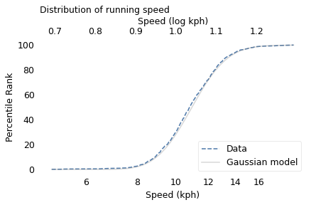
The logarithms follow a Gaussian distribution, which means the speeds themselves are lognormal. You might wonder why. Well, I have a theory, based on the following assumptions:

• First, everyone has a maximum speed they are capable of running, assuming that they train effectively.
• Second, these speed limits can depend on many factors, including height and weight, fast- and slow-twitch muscle mass, cardiovascular conditioning, flexibility and elasticity, and probably more.
• Finally, the way these factors interact tends to be multiplicative; that is, each person’s speed limit depends on the product of multiple factors.

Here’s why I think speed depends on a product rather than a sum of factors. If all of your factors are good, you are fast; if any of them are bad, you are slow. Mathematically, the operation that has this property is multiplication.

For example, suppose there are only two factors, measured on a scale from 0 to 1, and each person’s speed limit is determined by their product. Let’s consider three hypothetical people:

• The first person scores high on both factors, let’s say 0.9. The product of these factors is 0.81, so they would be fast.
• The second person scores relatively low on both factors, let’s say 0.3. The product is 0.09, so they would be quite slow.

So far, this is not surprising: if you are good in every way, you are fast; if you are bad in every way, you are slow. But what if you are good in some ways and bad in others?

• The third person scores 0.9 on one factor and 0.3 on the other. The product is 0.27, so they are a little bit faster than someone who scores low on both factors, but much slower than someone who scores high on both.

That’s a property of multiplication: the product depends most strongly on the smallest factor. And as the number of factors increases, the effect becomes more dramatic.

To simulate this mechanism, I generated five random factors from a Gaussian distribution and multiplied them together. I adjusted the mean and standard deviation of the Gaussians so that the resulting distribution fit the data; the following figure shows the results.

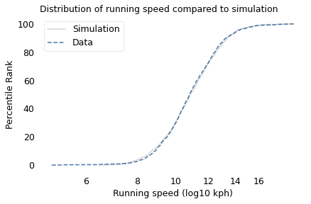
The simulation results fit the data well. So this example demonstrates a second mechanism that can produce lognormal distributions: the limiting power of the weakest link. If there are at least five factors that affect running speed, and each person’s limit depends on their worst factor, that would explain why the distribution of running speed is lognormal.

I suspect that distributions of many other skills are also lognormal, for similar reasons. Unfortunately, most abilities are not as easy to measure as running speed, but some are. For example, chess-playing skill can be quantified using the Elo rating system, which we’ll explore in the next section.

Chess Rankings

In the Elo chess rating system, every player is assigned a score that reflects their ability. These scores are updated after every game. If you win, your score goes up; if you lose, it goes down. The size of the increase or decrease depends on your opponent’s score. If you beat a player with a higher score, your score might go up a lot; if you beat a player with a lower score, it might barely change. Most scores are in the range from 100 to about 3000, although in theory there is no lower or upper bound.

By themselves, the scores don’t mean very much; what matters is the difference in scores between two players, which can be used to compute the probability that one beats the other. For example, if the difference in scores is 400, we expect the higher-rated player to win about 90% of the time.

If the distribution of chess skill is lognormal, and if Elo scores quantify this skill, we expect the distribution of Elo scores to be lognormal. To find out, I collected data from Chess.com, which is a popular internet chess server that hosts individual games and tournaments for players from all over the world. Their leader board shows the distribution of Elo ratings for almost six million players who have used their service. The following figure shows the distribution of these scores on a log scale, along with a lognormal model.

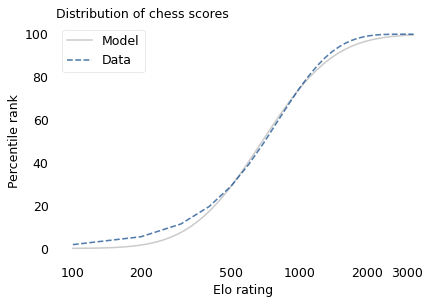
The lognormal model does not fit the data particularly well. But that might be misleading, because unlike running speeds, Elo scores have no natural zero point. The conventional zero point was chosen arbitrarily, which means we can shift it up or down without changing what the scores mean relative to each other.

With that in mind, suppose we shift the entire scale so that the lowest point is 550 rather than 100. The following figure shows the distribution of these shifted scores on a log scale, along with a lognormal model.

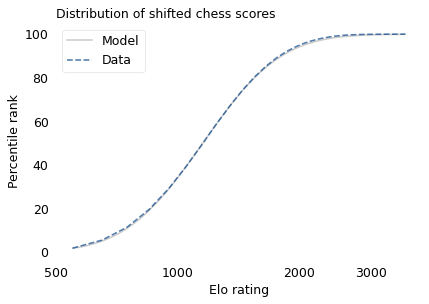
With this adjustment, the lognormal model fits the data well.

Now, we’ve seen two explanations for lognormal distributions: proportional growth and weakest links. Which one determines the distribution of abilities like chess? I think both mechanisms are plausible.

As you get better at chess, you have opportunities to play against better opponents and learn from the experience. You also gain the ability to learn from others; books and articles that are inscrutable to beginners become invaluable to experts. As you understand more, you are able to learn faster, so the growth rate of your skill might be proportional to your current level.

At the same time, lifetime achievement in chess can be limited by many factors. Success requires some combination of natural abilities, opportunity, passion, and discipline. If you are good at all of them, you might become a world-class player. If you lack any of them, you will not. The way these factors interact is like multiplication, where the outcome is most strongly affected by the weakest link.

These mechanisms shape the distribution of ability in other fields, even the ones that are harder to measure, like musical ability. As you gain musical experience, you play with better musicians and work with better teachers. As in chess, you can benefit from more advanced resources. And, as in almost any endeavor, you learn how to learn.

At the same time, there are many factors that can limit musical achievement. One person might have a bad ear or poor dexterity. Another might find that they don’t love music enough, or they love something else more. One might not have the resources and opportunity to pursue music; another might lack the discipline and tenacity to stick with it. If you have the necessary aptitude, opportunity, and personal attributes, you could be a world-class musician; if you lack any of them, you probably can’t.

Outliers

If you have read Malcolm Gladwell’s book, Outliers, this conclusion might be disappointing. Based on examples and research on expert performance, Gladwell suggests that it takes 10,000 hours of effective practice to achieve world-class mastery in almost any field.

Referring to a study of violinists led by the psychologist K. Anders Ericsson, Gladwell writes:

The striking thing […] is that he and his colleagues couldn’t find any ‘naturals,’ musicians who floated effortlessly to the top while practicing a fraction of the time their peers did. Nor could they find any ‘grinds,’ people who worked harder than everyone else, yet just didn’t have what it takes to break the top ranks.”

The key to success, Gladwell concludes, is many hours of practice. The source of the number 10,000 seems to be neurologist Daniel Levitin, quoted by Gladwell:

“In study after study, of composers, basketball players, fiction writers, ice skaters, concert pianists, chess players, master criminals, and what have you, this number comes up again and again. […] No one has yet found a case in which true world-class expertise was accomplished in less time.”

The core claim of the rule is that 10,000 hours of practice is necessary to achieve expertise. Of course, as Ericsson wrote in a commentary, “There is nothing magical about exactly 10,000 hours”. But it is probably true that no world-class musician has practiced substantially less.

However, some people have taken the rule to mean that 10,000 hours is sufficient to achieve expertise. In this interpretation, anyone can master any field; all they have to do is practice! Well, in running and many other athletic areas, that is obviously not true. And I doubt it is true in chess, music, or many other fields.

Natural talent is not enough to achieve world-level performance without practice, but that doesn’t mean it is irrelevant. For most people in most fields, natural attributes and circumstances impose an upper limit on performance.

In his commentary, Ericsson summarizes research showing the importance of “motivation and the original enjoyment of the activities in the domain and, even more important, […] inevitable differences in the capacity to engage in hard work (deliberate practice).” In other words, the thing that distinguishes a world-class violinist from everyone else is not 10,000 hours of practice, but the passion, opportunity, and discipline it takes to spend 10,000 hours doing anything.

The Greatest of All Time

Lognormal distributions of ability might explain an otherwise surprising phenomenon: in many fields of endeavor, there is one person widely regarded as the Greatest of All Time or the G.O.A.T.

For example, in hockey, Wayne Gretzky is the G.O.A.T. and it would be hard to find someone who knows hockey and disagrees. In basketball, it’s Michael Jordan; in women’s tennis, Serena Williams, and so on for most sports. Some cases are more controversial than others, but even when there are a few contenders for the title, there are only a few.

And more often than not, these top performers are not just a little better than the rest, they are a lot better. For example, in his career in the National Hockey League, Wayne Gretzky scored 2,857 points (the total of goals and assists). The player in second place scored 1,921. The magnitude of this difference is surprising, in part, because it is not what we would get from a Gaussian distribution.

To demonstrate this point, I generated a random sample of 100,000 people from a lognormal distribution loosely based on chess ratings. Then I generated a sample from a Gaussian distribution with the same mean and variance. The following figure shows the results.

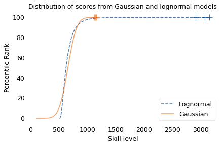
The mean and variance of these distributions is about the same, but the shapes are different: the Gaussian distribution extends a little farther to the left, and the lognormal distribution extends much farther to the right.

The crosses indicate the top three scorers in each sample. In the Gaussian distribution, the top three scores are 1123, 1146, and 1161. They are barely distinguishable in the figure, and and if we think of them as Elo scores, there is not much difference between them. According to the Elo formula, we expect the top player to beat the #3 player about 55% of the time.

In the lognormal distribution, the top three scores are 2913, 3066, and 3155. They are clearly distinct in the figure and substantially different in practice. In this example, we expect the top player to beat #3 about 80% of the time.

In reality, the top-rated chess players in the world are more tightly clustered than my simulated players, so this example is not entirely realistic. Even so, Garry Kasparov is widely considered to be the greatest chess player of all time. The current world champion, Magnus Carlsen, might overtake him in another decade, but even he acknowledges that he is not there yet.

Less well known, but more dominant, is Marion Tinsley, who was the checkers (aka draughts) world champion from 1955 to 1958, withdrew from competition for almost 20 years – partly for lack of competition – and then reigned uninterrupted from 1975 to 1991. Between 1950 and his death in 1995, he lost only seven games, two of them to a computer. The man who programmed the computer thought Tinsley was “an aberration of nature”.

Marion Tinsley might have been the greatest G.O.A.T. of all time, but I’m not sure that makes him an aberration. Rather, he is an example of the natural behavior of lognormal distributions:

• In a lognormal distribution, the outliers are farther from average than in a Gaussian distribution, which is why ordinary runners can’t beat the Freeze, even with a head start.
• And the margin between the top performer and the runner-up is wider than it would be in a Gaussian distribution, which is why the greatest of all time is, in many fields, an outlier among outliers.