The Raven Paradox
Suppose you are not sure whether all ravens are black. If you see a white raven, that clearly refutes the hypothesis. And if you see a black raven, that supports the hypothesis in the sense that it increases our confidence, maybe slightly. But what if you see a red apple – does that make the hypothesis any more or less likely?
This question is the core of the Raven paradox, a problem in the philosophy of science posed by Carl Gustav Hempel in the 1940s. It highlights a counterintuitive aspect of how we evaluate evidence and confirm hypotheses.
No resolution of the paradox is universally accepted, but the most widely accepted is what I will call the standard Bayesian response. In this article, I’ll present this response, explain why I think it is incomplete, and propose an extension that might resolve the paradox.
Click here to run this notebook on Colab.
The Problem
The paradox starts with the hypothesis
A: All ravens are black
And the contrapositive hypothesis
B: All non-black things are non-ravens
Logically, these hypotheses are identical – if A is true, B must be true, and vice versa. So if we have a certain level of confidence in A, we should have exactly the same confidence in B. And if we observe evidence in favor of A, we should also accept it as evidence in favor of B, to the same degree.
Also, if we accept that a black raven is evidence in favor of A, we should also accept that a non-black non-raven is evidence in favor of B.
Finally, if a non-black non-raven is evidence in favor of B, we should also accept that it is evidence in favor of A.
Therefore, a red apple (which is a non-black non-raven) is evidence that all ravens are black.
If you accept this conclusion, it seems like every time you see a red apple (or a blue car, or a green leaf, etc.) you should think, “Now I am slightly more confident that all ravens are black”.
But that seems absurd, so we have two options:
- Discover an error in the argument, or
- Accept the conclusion.
As you might expect, many versions of (1) and (2) have been proposed.
The standard Bayesian response is to accept the conclusion but, quoth Wikipedia “argue that the amount of confirmation provided is very small, due to the large discrepancy between the number of ravens and the number of non-black objects. According to this resolution, the conclusion appears paradoxical because we intuitively estimate the amount of evidence provided by the observation of a green apple to be zero, when it is in fact non-zero but extremely small.”
It is true that when the number of non-ravens is large, the amount of evidence we get from each non-black non-raven is so small it is negligible. But I don’t think that’s why the conclusion is so acutely counterintuitive.
To clarify my objection, let me present a smaller example I’ll call the Roulette paradox.
The Roulette Paradox
An American roulette wheel has 36 pockets with the numbers 1 to 36, and two pockets labeled 0 and 00. The non-zero pockets are red or black, and the zero pockets are green.
Suppose we work in quality control at the roulette factory and our job is to check that all zero pockets are green. If we observe a green zero, that’s evidence that all zeros are green. But what if we observe a red 19?
In this example, the standard Bayesian response fails:
- First, the number of non-zeros is not particularly large, so the weight of the evidence is not negligible.
- Also, the Bayesian response doesn’t address what I think is actually the key: The non-green non-zero may or may not be evidence, depending on how it was sampled.
As I will demonstrate,
- If we choose a pocket at random and it turns out to be a non-green non-zero, that is not evidence that all zeros are green.
- But if we choose a non-green pocket and it turns out to be non-zero, that is evidence that all zeros are green.
In both cases we observe a non-green non-zero, but “observe” is ambiguous. Whether the observation is evidence or not depends on the sampling process that generated the observation. And I think confusion between these two scenarios is the foundation of the paradox.
The Setup
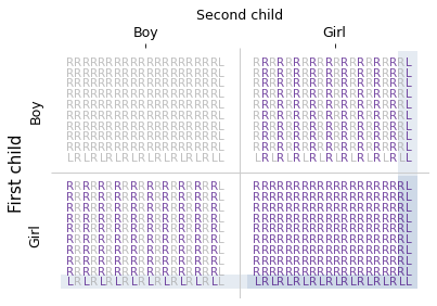
Let’s get into the details. Switching from roulette back to ravens, we will consider four scenarios:
- You choose a random thing and it turns out to be a black raven.
- You choose a random thing and it turns out to be a non-black non-raven.
- You choose a random raven and it turns out to be black.
- You choose a random non-black thing and it turns out to be a non-raven.
The key to the raven paradox is the difference between scenarios 2 and 4.
- Scenario 2 is what most people imagine when they picture “observing a red apple”. And in this scenario, the red apple is irrelevant, exactly as intuition insists.
- In Scenario 4, a red apple is evidence in favor of A, because we’re systematically checking non-black things to ensure they’re not ravens – so finding they aren’t is confirmation. But this sampling process is a more contrived interpretation of “observing a red apple”.
The reason for the paradox is that we imagine Scenario 2 and we are given the conclusion from Scenario 4.
It might not be obvious why the red apple is evidence in Scenario 4, but not Scenario 2. I think it will be clearer if we do the math.
The Math
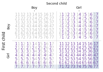
We’ll start with a small world where there are only N = 9 ravens and M = 19 non-ravens. Then we’ll see what happens as we vary N and M.
I’ll use i to represent the unknown number of black ravens, which could be any value from 0 to N, and j to represent the unknown number of black non-ravens, from 0 to M.
We’ll use a joint distribution to represent beliefs about i and j; then we’ll use Bayes’s Theorem to update these beliefs when we see new data.
Let’s start with a uniform prior over all possible combinations of (i, j). For this prior, the probability of A is 10%. We’ll see later that the prior affects the strength of the evidence, but it doesn’t affect whether an observation is in favor of A or not.
Scenario 1
Now let’s consider the first scenario: we choose a thing at random from the universe of things, and we find that it is a black raven.
The likelihood for this observation is: i / (N + M), because i is the number of black ravens and N + M is the total number of things.
In this scenario the posterior probability of A is 20%. The posterior probability is higher than the prior, so the black raven is evidence in favor of A.
To quantify the strength of the evidence, we’ll use the log odds ratio, which is 0.81. Later we’ll see how the strength of the evidence depends on the prior distribution of i and j.
Before we go on, let’s also look at the marginal distribution of i (number of black ravens) before and after.
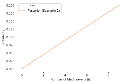
As expected, observing a black raven increases our confidence that all ravens are black. The posterior distribution shifts toward higher values of i, and the probability that i = N increases.
In Scenario 1, the likelihood depends only on i, not on j, so the update doesn’t change our beliefs about j (the number of black non-ravens).
Finally, let’s visualize posterior joint distribution of i and j.
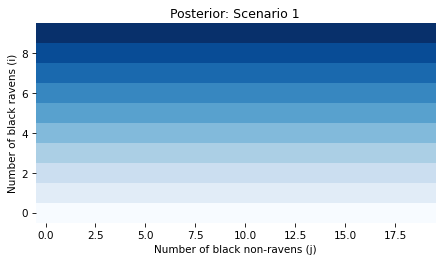
Because we started with a uniform distribution and the data has no bearing on j, the joint posterior probabilities don’t depend on j.
In summary, Scenario 1 is consistent with intuition: a black raven is evidence in favor of A.
Scenario 2
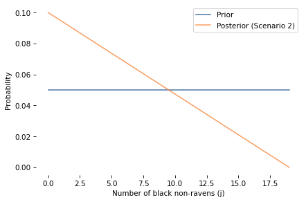
In this scenario, we choose a thing at random from the universe of N + M things, and it turns out to be a red apple – which we will treat generally as a non-black non-raven.
The likelihood of this observation is: (M - j) / (N + M), because M - j is the number of non-black non-ravens and N + M is the total number of things.
In this scenario, the posterior probability of A is the same as the prior. In fact, the entire distribution of i is unchanged.
So the red apple is not evidence in favor of A or against it. This is consistent with the intuition that the red apple (or any non-black non-raven) is irrelevant.
However, the red apple is evidence about j, as we can confirm by comparing the marginal distribution of j before and after.
And here’s the posterior joint distribution of i and j.
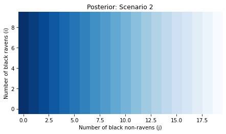
Because the red apple has no bearing on i, the posterior probabilities in this scenario don’t depend on i.
In summary, Scenario 2 matches our intuition: a red apple (chosen at random) is not evidence about whether all ravens are black.
Scenario 3
In this scenario, we choose a raven first and then observe that it is black.
The likelihood for this observation is: i / N, because i is the number of black ravens and N is the total number of ravens.
In this scenario, the posterior probability of A is 20%, the same as in Scenario 1.So we conclude that the black raven is evidence in favor of A, with the same strength regardless of whether we are in:
- Scenario 1: Select a random thing and it turns out to be a black raven or
- Scenario 3: Select a random raven and it turns out to be black.
In fact, the entire posterior distribution is the same in both scenarios. That’s because the likelihoods in Scenarios 1 and 3 differ only by a constant factor, which is removed when the posterior distributions are normalized.
In summary, Scenario 3 is consistent with intuition: if we choose a raven and find that it is black, that is evidence in favor of A.
Scenario 4
In the last scenario, we first choose a non-black thing (from all non-black things in the universe), and then observe that it is a non-raven.
The likelihood of this observation is: (M - j) / (N - i + M - j) because M - j is the number of non-black non-ravens and N - i + M - j is the total number of non-black things.
This likelihood depends on both i and j, unlike Scenario 2. This is the key difference that makes Scenario 4 informative about whether all ravens are black.
The posterior probability of A is about 15%, which is greater than the prior, so the non-black non-raven is evidence in favor of A. The log odds ratio is about 0.47, which is smaller than in Scenarios 1 and 3, because there are more non-ravens than ravens. As we’ll see, the strength of the evidence gets smaller as M gets bigger.
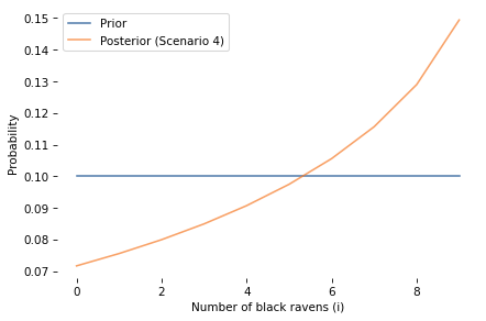
Here is the marginal distribution of i (number of black ravens) before and after.
And here’s the marginal distribution of j (number of black non-ravens) before and after.
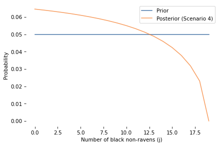
Finally, here’s the posterior joint distribution of i and j.
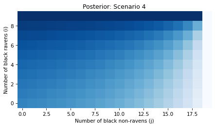
In Scenario 4, the likelihood depends on both i and j, so the update changes our beliefs about both parameters.
And in Scenario 4 a non-black non-raven (chosen from non-black things) is evidence in favor of A. This might still be surprising, but let me suggest a way to think about it: in this scenario we are checking non-black things to make sure they are not ravens. If we find a non-black raven, that contradicts A. If we don’t, that supports A.
In all four scenarios, the results are consistent with intuition. So as long as you are clear about which scenario you are in, there is no paradox. The paradox is only apparent if you think you are in Scenario 2 and you imagine the result from Scenario 4.
In the context of the original problem:
- If you walk out of your house and the first thing you see is a red apple (or a blue car, or a green leaf) that has no bearing on whether raven are black.
- But if you deliberately select a non-black thing and check whether it’s a raven, and you find that it is not, that actually is evidence that all ravens are black – but consistent with the standard Bayesian response, it is so weak it is negligible.
Successive updates
In these examples, we started with a uniform prior over all combinations of i and j. Of course that’s not a realistic representation of what we believe about the world. So let’s consider the effect of other priors.
In general, different priors lead to different posterior distributions, and in this case they lead to different conclusions about the strength of the evidence. But they lead to the same conclusion about the direction of the evidence.
To demonstrate, let’s see what happens if we observe a series of black ravens (in Scenario 1 or 3). For simplicity, assume that we sample with replacement.
The following function computes multiple updates, starting with the uniform prior and then using the posterior from each update as the prior for the next.
This table shows the results in Scenario 1 (which is the same as in Scenario 3). For each iteration, the table shows the prior and posterior probability of A, and the log odds ratio.
| Iteration | Prior | Posterior | LOR |
|---|---|---|---|
| 0 | 0.100000 | 0.200000 | 0.810930 |
| 1 | 0.200000 | 0.284211 | 0.462624 |
| 2 | 0.284211 | 0.360000 | 0.348307 |
| 3 | 0.360000 | 0.427901 | 0.284942 |
| 4 | 0.427901 | 0.488715 | 0.245274 |
| 5 | 0.488715 | 0.543171 | 0.218261 |
| 6 | 0.543171 | 0.591920 | 0.198796 |
| 7 | 0.591920 | 0.635551 | 0.184196 |
| 8 | 0.635551 | 0.674590 | 0.172914 |
| 9 | 0.674590 | 0.709512 | 0.163995 |
As we see more ravens, the posterior probability of A increases, but the LOR decreases – which means that each raven provides weaker evidence than the previous one. In the long run the LOR converges to a value greater than 0 (about 0.11), which means that each raven provides at least some additional evidence, even when the prior is far from the uniform distribution we started with.
In the worst case, if the prior probability of A is 0 or 1, nothing we observe can change those beliefs, so nothing is evidence for or against A. But there is no prior where a black raven provides evidence against A.
[Proof: The likelihood of the observation is maximized when all ravens are black (i = N). Therefore, for any prior that gives non-zero probability to both A and its complement, the LOR is positive: these observations can never be evidence against A.]
The following table shows the results in Scenario 4, where we select a non-black thing and check that it is not a raven.
| Iteration | Prior | Posterior | LOR |
|---|---|---|---|
| 0 | 0.100000 | 0.149403 | 0.457933 |
| 1 | 0.149403 | 0.201006 | 0.359272 |
| 2 | 0.201006 | 0.253991 | 0.302582 |
| 3 | 0.253991 | 0.307217 | 0.264273 |
| 4 | 0.307217 | 0.359496 | 0.235611 |
| 5 | 0.359496 | 0.409837 | 0.212911 |
| 6 | 0.409837 | 0.457528 | 0.194344 |
| 7 | 0.457528 | 0.502141 | 0.178860 |
| 8 | 0.502141 | 0.543477 | 0.165785 |
| 9 | 0.543477 | 0.581514 | 0.154644 |
The pattern is similar. Each non-black thing that turns out not to be a raven is weaker evidence than the previous one. But it is always in favor of A – in this scenario, there is no prior where a non-black non-raven is evidence against A.
Varying M
Finally, let’s see how the strength of the evidence varies as we increase M, the number of non-ravens. The following function computes results in Scenario 4 for a range of values of M, holding constant the number of ravens, N = 9.
| M | Prior | Posterior | LOR |
|---|---|---|---|
| 20 | 0.1 | 0.147655 | 0.444110 |
| 50 | 0.1 | 0.124515 | 0.246875 |
| 100 | 0.1 | 0.114530 | 0.151946 |
| 200 | 0.1 | 0.108495 | 0.091022 |
| 500 | 0.1 | 0.104100 | 0.044751 |
| 1000 | 0.1 | 0.102331 | 0.025640 |
As M increases (more non-ravens in the universe), the strength of the evidence decreases. This is consistent with the standard Bayesian response, which notes that in a realistic scenario, the evidence is negligible.
Conclusion
The standard Bayesian response to the Raven paradox is correct in the sense that if a non-black non-raven is evidence that all ravens are black, it is so extremely weak. But that doesn’t explain why the roulette example – where the number of non-green non-zero pockets is relatively small – is still so contrary to intuition.
I think a better explanation for the paradox is the ambiguity of the word “observe”. If we are explicit about the sampling process that generates the observation, we find that a non-black non-raven may or may not be evidence that all ravens are black.
- Scenario 2: If we choose a random thing and find that it is a non-black non-raven, that is not evidence.
- Scenario 4: If we choose a non-black thing and find that it is a non-raven, that is evidence.
The first case is entirely consistent with intuition. The second case is less obvious, but if we consider smaller examples like a roulette wheel, and do the math, it can be reconciled with intuition.
Confusion between these scenarios causes the apparent paradox, and clarity about the scenarios resolves it.
Symmetry and Asymmetry
It might still seem strange that a black raven is always evidence for A and B, but a non-black non-raven may or may not be, depending on the sampling process. If A and B are logically identical, and a black raven supports A, it’s still not clear why a non-black non-raven doesn’t always support B.
After all, if we start with B, we conclude that a non-black non-raven is always evidence for B (and A), and a black raven may or may not be. Where does this asymmetry come from?
We broke the symmetry when we formulated “All ravens are black” as “Out of all ravens, how many are black?” This formulation first divides the world into ravens and non-ravens, then asks how many in each group are black.
Conversely, if we start with “All non-black things are non-ravens”, we formulate it as “Out of all non-black things, how many are ravens?” In this formulation, we divide the world into black and non-black things, then ask how many in each group are ravens.
The asymmetry is apparent when we parameterize the models. If we start with A, we define i to be the number of ravens that are black. And we find that in Scenario 1, the likelihood of a black raven depends on i, and in Scenario 2, the likelihood of a non-black non-raven does not.
If we start with B, we define i to be the number of non-black things that are non-ravens. Then in Scenario 1 we find that a non-black non-raven pertains to i, but a black raven does not.
So the symmetry is broken when we formulate the hypothesis in a way that is testable with data. In propositional logic, A and B are equivalent in the sense that evidence for one must be evidence for the other. In the Bayesian formulation, “How many ravens are black?” and “How many non-black things are non-ravens?” are not equivalent; evidence for one is not necessarily evidence for the other.
A critic might say that the Bayesian formulation is a non-resolution – that is, it doesn’t solve the original problem posed by Hempel; it only solves a related problem by making additional assumptions.
A Bayesian response is that the Raven Paradox is only problematic in the abstract world of propositional logic; as soon as we formulate the question in a way that connects it to the real world through observation, it disappears. So the Raven Paradox is similar to the principle of explosion – it demonstrates a brittleness in propositional logic that makes it unsuitable for reasoning about many real-world hypotheses.
Related Reading
I am not the first to notice that the interpretation of evidence depends on a model of the data-generating process. In the context of the Raven Problem, Richard Royall wrote:
We see that the observation of a red pencil can be evidence that all ravens are black. To make the proper interpretation, we must have an additional piece of information. Whether the observation is or is not evidence supporting the hypothesis (A) that all ravens are black versus the hypothesis (B) that only a fraction … are black is determined by the sampling procedure. A randomly selected pencil that proves to be red is not evidence that all ravens are black, but a randomly selected red object that proves to be a pencil is.
This analysis appears in an appendix of Statistical evidence: a likelihood paradigm, first published in 1997. I found it in a footnote of Belief, Evidence, and Uncertainty: Problems of Epistemic Inference, published in 2016:
Royall in his commentary on the Raven Paradox … observes that how one got the white shoes is inferentially important. If you grabbed a non-raven object at random, then it does not bear on the question of whether all ravens are black. If on the other hand you grabbed a random non-black object, and it turned out to be a pair of shoes, then it provides a very tiny amount of evidence for the hypothesis that all ravens are black …
Royall is right that the sampling process determines whether a red pencil (or white shoe) is evidence about ravens, and he analyzes a version of what I’m calling Scenario 4. But I don’t think his analysis quite explains why the paradox feels so counterintuitive, and it seems to have had little impact on the discussion of the Raven paradox in the confirmation theory literature.
Here is a longer version of this article that includes all of the code and a list of objections with my responses. You can also click here to run the notebook on Colab.