Watch your tail!
For a long time I have recommended using CDFs to compare distributions. If you are comparing an empirical distribution to a model, the CDF gives you the best view of any differences between the data and the model.
Now I want to amend my advice. CDFs give you a good view of the distribution between the 5th and 95th percentiles, but they are not as good for the tails.
To compare both tails, as well as the “bulk” of the distribution, I recommend a triptych that looks like this:
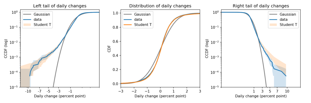
There’s a lot of information in that figure. So let me explain.
The code for this article is in this Jupyter notebook.
Daily changes
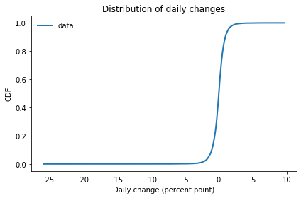
Suppose you observe a random process, like daily changes in the S&P 500. And suppose you have collected historical data in the form of percent changes from one day to the next. The distribution of those changes might look like this:
If you fit a Gaussian model to this data, it looks like this:
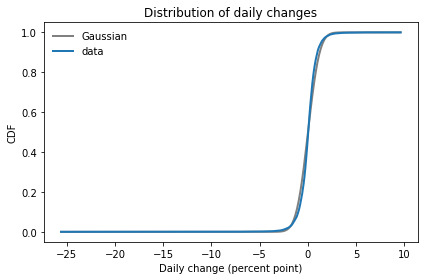
It looks like there are small discrepancies between the model and the data, but if you follow my previous advice, you might look at these CDFs and conclude that the Gaussian model is pretty good.
If we zoom in on the middle of the distribution, we can see the discrepancies more clearly:
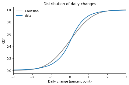
In this figure it is clearer that the Gaussian model does not fit the data particularly well. And, as we’ll see, the tails are even worse.
Survival on a log-log scale
In my opinion, the best way to compare tails is to plot the survival curve (which is the complementary CDF) on a log-log scale.
In this case, because the dataset includes positive and negative values, I shift them right to view the right tail, and left to view the left tail.
Here’s what the right tail looks like:
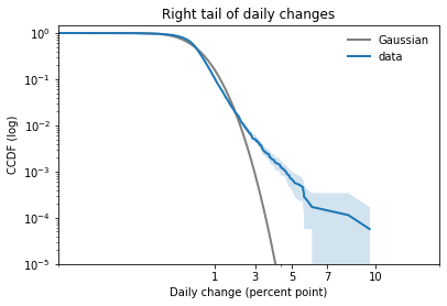
This view is like a microscope for looking at tail behavior; it compresses the bulk of the distribution and expands the tail. In this case we can see a small discrepancy between the data and the model around 1 percentage point. And we can see a substantial discrepancy above 3 percentage points.
The Gaussian distribution has “thin tails”; that is, the probabilities it assigns to extreme events drop off very quickly. In the dataset, extreme values are much more common than the model predicts.
The results for the left tail are similar:
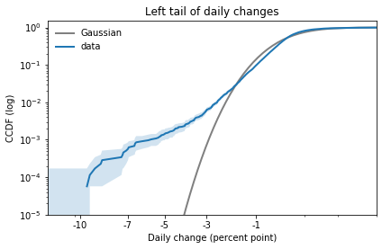
Again, there is a small discrepancy near -1 percentage points, as we saw when we zoomed in on the CDF. And there is a substantial discrepancy in the leftmost tail.
Student’s t-distribution
Now let’s try the same exercise with Student’s t-distribution. There are two ways I suggest you think about this distribution:
1) Student’s t is similar to a Gaussian distribution in the middle, but it has heavier tails. The heaviness of the tails is controlled by a third parameter, ν.
2) Also, Student’s t is a mixture of Gaussian distributions with different variances. The tail parameter, ν, is related to the variance of the variances.
For a demonstration of the second interpretation, I recommend this animation by Rasmus Bååth.
I used PyMC to estimate the parameters of a Student’s t model and generate a posterior predictive distribution. You can see the details in this Jupyter notebook.
Here is the CDF of the Student t model compared to the data and the Gaussian model:
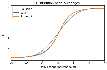
In the bulk of the distribution, Student’s t-distribution is clearly a better fit.
Now here’s the right tail, again comparing survival curves on a log-log scale:
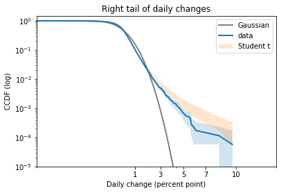
Student’s t-distribution is a better fit than the Gaussian model, but it overestimates the probability of extreme values. The problem is that the left tail of the empirical distribution is heavier than the right. But the model is symmetric, so it can only match one tail or the other, not both.
Here is the left tail:
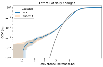
The model fits the left tail about as well as possible.
If you are primarily worried about predicting extreme losses, this model would be a good choice. But if you need to model both tails well, you could try one of the asymmetric generalizations of Student’s t.
The old six sigma
The tail behavior of the Gaussian distribution is the key to understanding “six sigma events”.
John Cook explains six sigmas in this excellent article:
“Six sigma means six standard deviations away from the mean of a probability distribution, sigma (σ) being the common notation for a standard deviation. Moreover, the underlying distribution is implicitly a normal (Gaussian) distribution; people don’t commonly talk about ‘six sigma’ in the context of other distributions.”
This is important. John also explains:
“A six-sigma event isn’t that rare unless your probability distribution is normal… The rarity of six-sigma events comes from the assumption of a normal distribution more than from the number of sigmas per se.”
So, if you see a six-sigma event, you should probably not think, “That was extremely rare, according to my Gaussian model.” Instead, you should think, “Maybe my Gaussian model is not a good choice”.