If you like this article, you can read more about this kind of Bayesian analysis in Think Bayes.

Recently I found a copy of Probably Overthinking It at a local bookstore and posted a picture on Twitter. Aubrey Clayton replied with this question:

It’s a great question with what turns out to be an interesting answer. I’ll summarize the results here, but if you want to see the calculations, you can run the notebook on Colab.

Assumptions

Suppose you are the author of a book like Probably Overthinking It, and when you visit a local bookstore, like Newtonville Books in Newton, MA, you see that they have two copies of your book on display.

Is it good that they have only a few copies, because it suggests they started with more and sold some? Or is it bad because it suggests they only keep a small number in stock, and they have not sold. More generally, what number of books would you like to see?

To answer these questions, we have to make some modeling decisions. To keep it simple, I’ll assume:

• The bookstore orders books on some regular cycle of unknown duration.
• At the beginning of every cycle, they start with k books.
• People buy the book at a rate of λ books per cycle.
• When you visit the store, you arrive at a random time t during the cycle.

We’ll start by defining prior distributions for these parameters, and then we’ll update it with the observed data.

Priors

For some books, the store only keeps one copy in stock. For others it might keep as many as ten. If we would be equally unsurprised by any value in this range, the prior distribution of k is uniform between 1 and 10.

If we arrive at a random point in the cycle, the prior distribution of t is uniform between 0 and 1, measured in cycles.

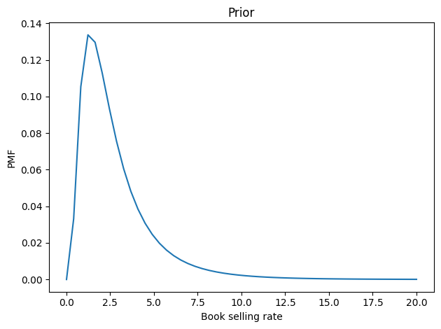
Now let’s figure the book-buying rate is probably between 2 and 3 copies per cycle, but it could be substantially higher – with low probability. We can choose a lognormal distribution that has a mean and shape that seem reasonable. Here’s what it looks like.

From these marginal prior distributions, we can form the joint prior. Now let’s update it.

The update

Now for the update, we have to handle two cases:

• If we observe at least one book, n, the probability of the data is the probability of selling k-n books at rate λ over period t, which is given by the Poisson PMF.
• If there are no copies left, we have to add in the probability that the number of books sold in this period could have exceeded k, which is given by the Poisson survival function.

After computing these likelihoods for all possible sets of parameters, we do a Bayesian update in the usual way, multiplying the priors by the likelihoods and normalizing the result.

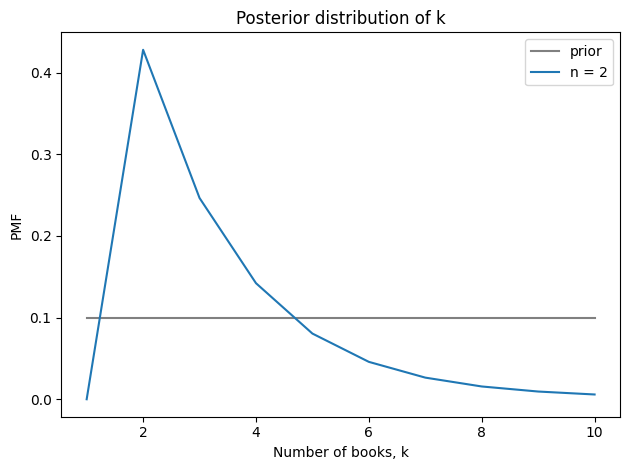
As an example, we’ll do an update with the hypothetically observed 2 books. Then, from the joint posterior, we can extract the marginal distributions of k and λ, and compute their means.

Seeing two books suggests that the store starts each cycle with 3-4 books and sells 2-3 per cycle. Here’s the posterior distribution of k compared to its prior.

And here’s the posterior distribution of λ.

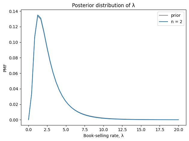
Seeing two books doesn’t provide much information about the book-selling rate.

Optimization

Now let’s consider the more general question, “What number of books would you most like to see?” There are two ways we might answer:

• One answer might be the observation that leads to the highest estimate of λ. But if the book-selling rate is high, relative to k, the book will sometimes be out of stock, leading to lost sales.
• So an alternative is to choose the observation that implies the highest number of books sold per cycle.

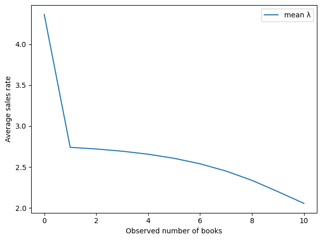
Computing the second is a little tricky — you can see the details in the notebook. But with that problem solved, we can loop over possible values of n and compute for each one the posterior mean values of λ and the implied number of books sold per cycle.

Here’s the implied sales rate as a function of the observed number of books. By this metric, the best number of books to see is 0.

And here’s the implied number of books sold per cycle.

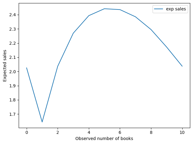
This result is a little more interesting. Seeing 0 books is still good, but the optimal value is around 5. The worst possibility is to see just one book.

Now, we should not take these values too literally, as they are based on a very small amount of data and a lot of assumptions – both in the model and in the priors. But it is interesting that the optimal point is neither 0 nor “as many as possible.

Thanks again to Aubrey Clayton for asking such an interesting question. If you are interesting in the history and future of statistical thinking, you might like his book, Bernoulli’s Fallacy.

previous