In honor of NASA’s successful DART mission, here’s a relevant excerpt from my forthcoming book, Probably Overthinking It.

On March 11, 2022, an astronomer near Budapest, Hungary detected a new asteroid, now named 2022 EB5, on a collision course with Earth. Less than two hours later, it exploded in the atmosphere near Greenland. Fortunately, no large fragments reached the surface, and they caused no damage.

We have not always been so lucky. In 1908, a much larger asteroid entered the atmosphere over Siberia, causing an estimated 2 megaton explosion, about the same size as the largest thermonuclear device tested by the United States. The explosion flattened something like 80 million trees in an area covering 2100 square kilometers, almost the size of Rhode Island. Fortunately, the area was almost unpopulated; a similar-sized impact could destroy a large city.

These events suggest that we would be wise to understand the risks we face from large asteroids. To do that, we’ll look at evidence of damage they have done in the past: the impact craters on the Moon.

The largest crater on the near side of the moon, named Bailly, is 303 kilometers in diameter; the largest on the far side, the South Pole-Aitken basin, is roughly 2500 kilometers in diameter.

In addition to large, visible craters like these, there are innumerable smaller craters. The Lunar Crater Database catalogs nearly all of the ones larger than one kilometer, about 1.3 million in total. It is based on images taken by the Lunar Reconnaissance Orbiter, which NASA sent to the Moon in 2009.

The following figures show the distribution of their sizes on a log scale, compared to a lognormal model. The left figure shows the tail distribution on a linear scale; the right figure shows the same curve on a log scale.

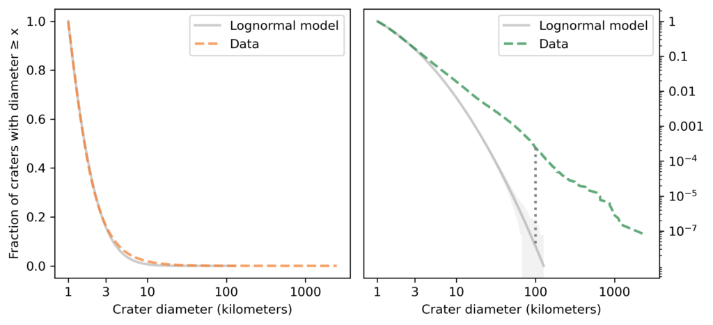
Since the dataset does not include craters smaller than one kilometer, I cut off the model at the same threshold. We can assume that there are many smaller craters, but with this dataset we can’t tell what the distribution of their sizes looks like.

Looking at the figure on the left, we can see a discrepancy between the data and the model between 3 and 10 kilometers. Nevertheless, the model fits the logarithms of the diameters well, so we could conclude that the distribution of crater sizes is approximately lognormal.

However, looking at the figure on the right, we can see big differences between the data and the model in the tail. In the dataset, the fraction of craters as big as 100 kilometers is about 250 per million; according to the model, it would be less than 1 per million. The dotted line in the figure shows this difference.

Going farther into the tail, the fraction of craters as big as 1000 kilometers is about 3 per million; according to the model, it would be less than one per trillion. And the probability of a crater as big as the South Pole-Aitken basin is about 50 per sextillion.

If we are only interested in craters less than 10 kilometers in diameter, the lognormal model might be good enough. But for questions related to the biggest craters, it is way off.

The following figure shows the distribution of crater sizes again, compared to a log-t model [which is the abbreviated name I use for a Student-t distribution on a log scale].

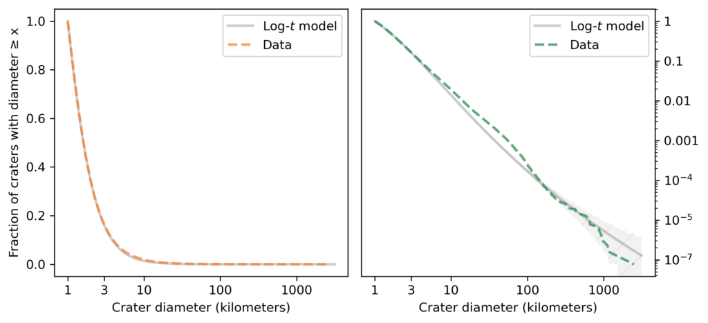
The figure on the left shows that the model fits the data well in the middle of the distribution, a little better than the lognormal model. The figure on the right shows that the log-t model fits the tail of the distribution substantially better than the lognormal model.

It’s not perfect: there are more craters near 100 km than the model expects, and fewer craters larger than 1000 km. As usual, the world is under no obligation to follow simple rules, but this model does pretty well.

We might wonder why. To explain the distribution of crater sizes, it helps to think about where they come from. Most of the craters on the Moon were formed during a period in the life of the solar system called the “Late Heavy Bombardment”, about 4 billion years ago. During this period, an unusual number of asteroids were displaced from the asteroid belt – possibly by interactions with large outer planets – and some of them collided with the Moon.

We assume that some of them also collided with the Earth, but none of the craters they made still exist; due to plate tectonics and volcanic activity, the surface of Earth has been recycled several times since the Late Heavy Bombardment.

But the Moon is volcanically inert and it has no air or water to erode craters away, so its craters are visible now in almost the same condition they were 4 billion years ago (with the exception of some that have been disturbed by later impacts and lunar spacecraft).

Asteroids

As you might expect, there is a relationship between the size of an asteroid and the size of the crater it makes: in general, a bigger asteroid makes a bigger crater. So, to understand why the distribution of crater sizes is long-tailed, let’s consider the distribution of asteroid sizes.

The Jet Propulsion Laboratory (JPL) and NASA provide data related to asteroids, comets and other small bodies in our solar system. From their Small-Body Database, I selected asteroids in the “main asteroid belt” between the orbits of Mars and Jupiter.

There are more than one million asteroids in this dataset, about 136,000 with known diameter. The largest are Ceres (940 kilometers in diameter), Vesta (525 km), Pallas (513 km), and Hygeia (407 km). The smallest are less than one kilometer.

The following figure shows the distribution of asteroid sizes compared to a lognormal model.

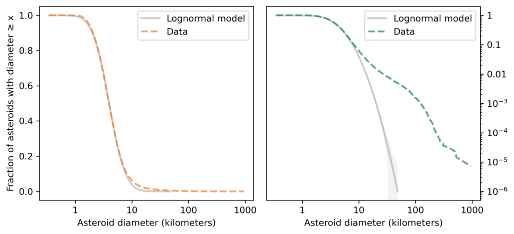
As you might expect by now, the lognormal model fits the distribution of asteroid sizes in the middle of the range, but it does not fit the tail at all. Rather than belabor the point, let’s get to the log-t model, as shown in the following figure.

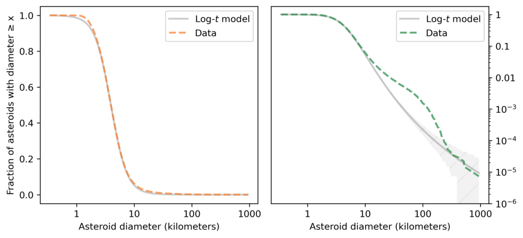
On the left, we see that the log-t model fits the data well near the middle of the range, except possibly near 1 kilometer.

On the right, we see that the model does not fit the tail of the distribution particularly well: there are more asteroids near 100 km than the model predicts. So the distribution of asteroid sizes does not strictly follow a log-t distribution. Nevertheless, it is clearly longer-tailed than a lognormal distribution, and we can use it to explain the distribution of crater sizes, as I’ll show in the next section.

Origins of Long-Tailed Distributions

One of the reasons long-tailed distributions are common in natural systems is that they are persistent; for example, if a quantity comes from a long-tailed distribution and you multiply it by a constant or raise it to a power, the result follows a long-tailed distribution.

Long-tailed distributions also persist when they interact with other distributions. When you add together two quantities, if either comes from a long-tailed distribution, the sum follows a long-tailed distribution, regardless of what the other distribution looks like. Similarly, when you multiply two quantities, if either comes from a long-tailed distribution, the product usually follows a long-tailed distribution. This property might explain why the distribution of crater sizes is long-tailed.

Empirically – that is, based on data rather than a physical model – the diameter of an impact crater depends on the diameter of the projectile that created it, raised to the power 0.78, and on the impact velocity raised to the power 0.44. It also depends on the density of the asteroid and the angle of impact.

As a simple model of this relationship, I’ll simulate the crater formation process by drawing asteroid diameters from the distribution in the previous section and drawing the other factors – density, velocity, and angle – from a lognormal distribution with parameters chosen to match the data. The following figure shows the results from this simulation along with the actual distribution of crater sizes.

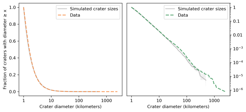
In the center of the distribution (left) and in the tail (right), the simulation results are a good match for the data. This example suggests that the distribution of crater sizes can be explained by the relationship between the distributions of asteroid sizes and other factors like velocity and density.

In turn, there are physical models that might explain the distribution of asteroid sizes. Our best current understanding is that the asteroids in the asteroid belt were formed by dust particles that collided and stuck together. This process is called “accretion”, and simple models of accretion processes can yield long-tailed distributions.

So it may be that craters are long-tailed because of asteroids, and asteroids are long-tailed because of accretion.

In The Fractal Geometry of Nature, Benoit Mandelbrot proposes what he calls a “heretical” explanation for the prevalence of long-tailed distributions in natural systems: there may be only a few systems that generate long-tailed distributions, but interactions between systems might cause them to propagate.

He suggests that data we observe are often “the joint effect of a fixed underlying true distribution and a highly variable filter”, and “a wide variety of filters leave their asymptotic behavior unchanged”.

The long tail in the distribution of asteroid sizes is an example of “asymptotic behavior”. And the relationship between the size of an asteroid and the size of the crater it makes is an example of a “filter”. In this relationship, the size of the asteroid gets raised to a power and multiplied by a “highly-variable” lognormal distribution. These operations change the location and spread of the distribution, but they don’t change the shape of the tail.

When Mandelbrot wrote in the 1970s, this explanation might have been heretical, but now long-tailed distributions are more widely known and better understood. What was heresy then is orthodoxy now.