Where’s My Train?
Yesterday I presented a webinar for PyMC Labs where I solved one of the exercises from Think Bayes, called “The Red Line Problem”. Here’s the scenario:
The Red Line is a subway that connects Cambridge and Boston, Massachusetts. When I was working in Cambridge I took the Red Line from Kendall Square to South Station and caught the commuter rail to Needham. During rush hour Red Line trains run every 7-8 minutes, on average.
When I arrived at the subway stop, I could estimate the time until the next train based on the number of passengers on the platform. If there were only a few people, I inferred that I just missed a train and expected to wait about 7 minutes. If there were more passengers, I expected the train to arrive sooner. But if there were a large number of passengers, I suspected that trains were not running on schedule, so I expected to wait a long time.
While I was waiting, I thought about how Bayesian inference could help predict my wait time and decide when I should give up and take a taxi.
I used this exercise to demonstrate a process for developing and testing Bayesian models in PyMC. The solution uses some common PyMC features, like the Normal, Gamma, and Poisson distributions, and some less common features, like the Interpolated and StudentT distributions.
The video is on YouTube now:
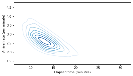
This talk will be remembered for the first public appearance of the soon-to-be-famous “Banana of Ignorance”. In general, when the data we have are unable to distinguish between competing explanations, that uncertainty is reflected in the joint distribution of the parameters. In this example, if we see more people waiting than expected, there are two explanation: a higher-than-average arrival rate or a longer-than-average elapsed time since the last train. If we make a contour plot of the joint posterior distribution of these parameters, it looks like this:

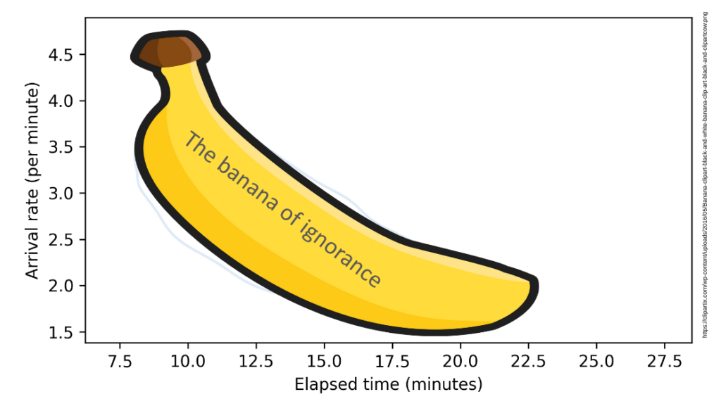
The elongated shape of the contour indicates that either explanation is sufficient: if the arrival rate is high, elapsed time can be normal, and if the elapsed time is high, the arrival rate can be normal. Because this shape indicates that we don’t know which explanation is correct, I have dubbed it “The Banana of Ignorance”:

For all of the details, you can read the Jupyter notebook or run it on Colab.
The original Red Line Problem is based on a student project from my Bayesian Statistics class at Olin College, way back in Spring 2013.