Someone asked me recently why I stopped writing about religion, and I said there were two reasons: One is that the primary dataset I was following

stopped updating; the other is that Ryan Burge is doing such a good job, I felt redundant.

His most recent article

presents evidence that the Nones have hit a ceiling — that is, that the percentage of people in the U.S. with no religious affiliation, which has consistently increased for several decades, has either leveled off or started to reverse.

He reports on new data from the Cooperative Election Study and the 2024 General Social Survey, including this figure based on the GSS.

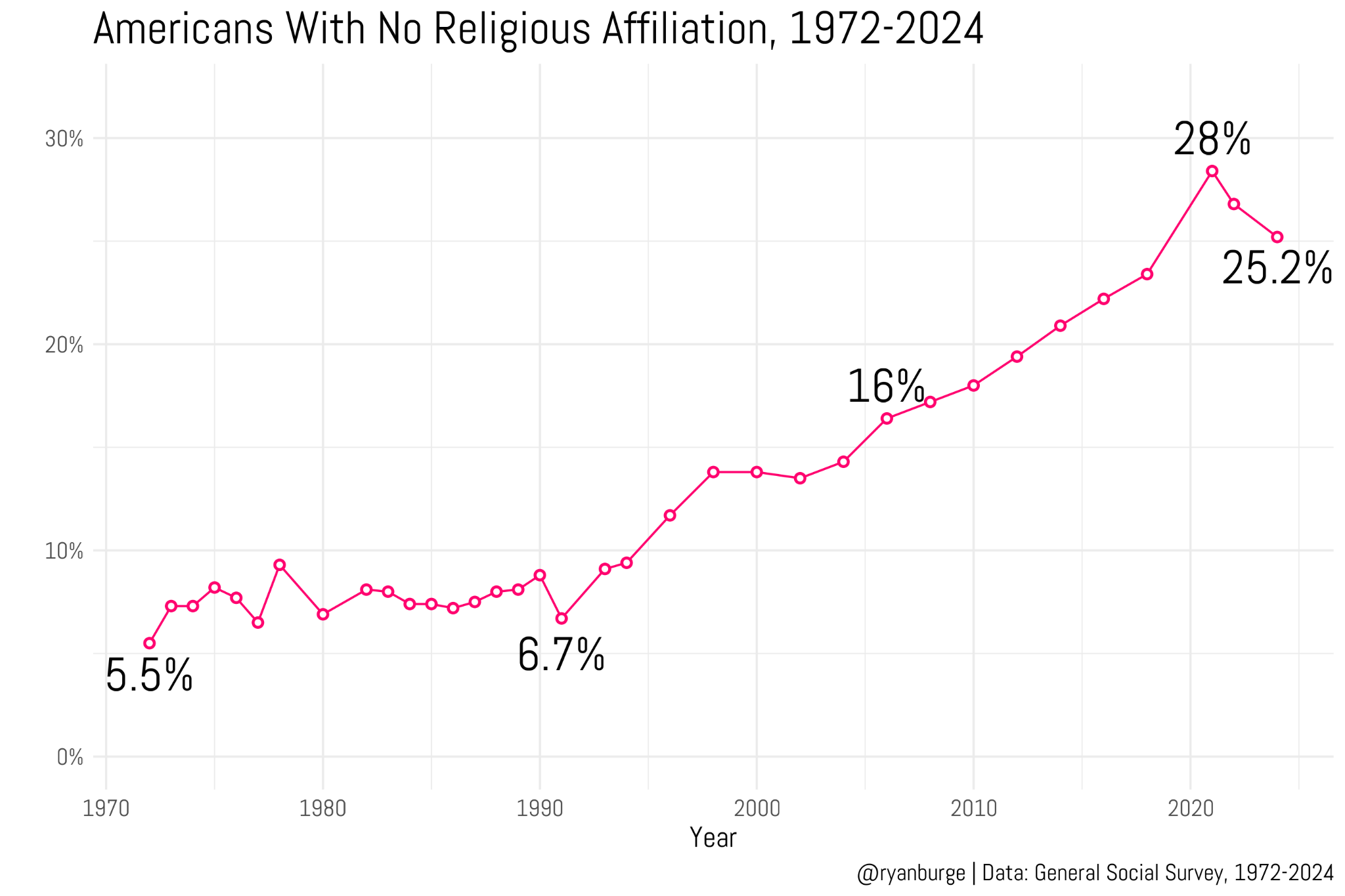
The percentage of “Nones” from Ryan Burge’s Graphs About Religion

.

The observed percentage of Nones peaked in the 2021 survey and has dropped in the last two cycles. The CES data show a similar pattern, with a much larger sample size. So I’m not going to disagree with Ryan: it sure looks like the rise of the Nones has stalled or even reversed.

However, since I am developing a model that decomposes trends like this into cohort and period effects, we can use it to check whether the turnaround is a cohort or a period effect. It turns out to be both.

The Model

The model assumes that each cohort in each year has an unobserved (latent) propensity to report a religious affiliation or none.

The cohort and period effects are modeled as second-order Gaussian random walks, which means the model assumes these effects evolve smoothly over time, unless the data provide strong evidence otherwise. The amount of smoothing is estimated from the data.

An additional random year effect captures variation from one survey to the next that is not explained by long-term trends, like current events and topics of discussion.

The “time only” version of the model estimates a latent propensity for each cycle of the survey, so the result is a smooth curve through the raw proportions.

The “time-cohort” version estimates a latent propensity for each cohort during each cycle, so the result is a trajectory over time for each birth year.

Results

Here are the results for the time-only model, showing the posterior mean and a 94% credible interval.

Time-only model, percent with no religious preference

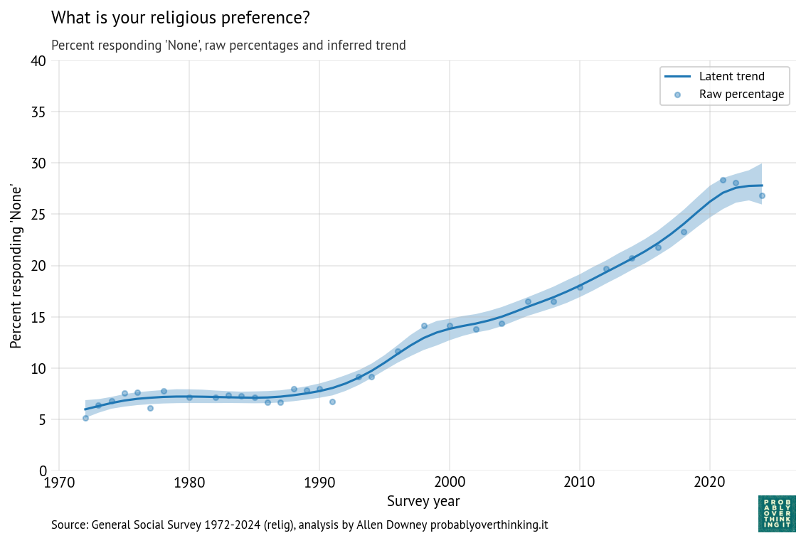
The posterior mean indicates that the trend in the latent factor has probably slowed; the credible interval indicates that it might have leveled off or reversed.

And here are the trajectories for each cohort:

Cohort trajectories, percent with no religious preference

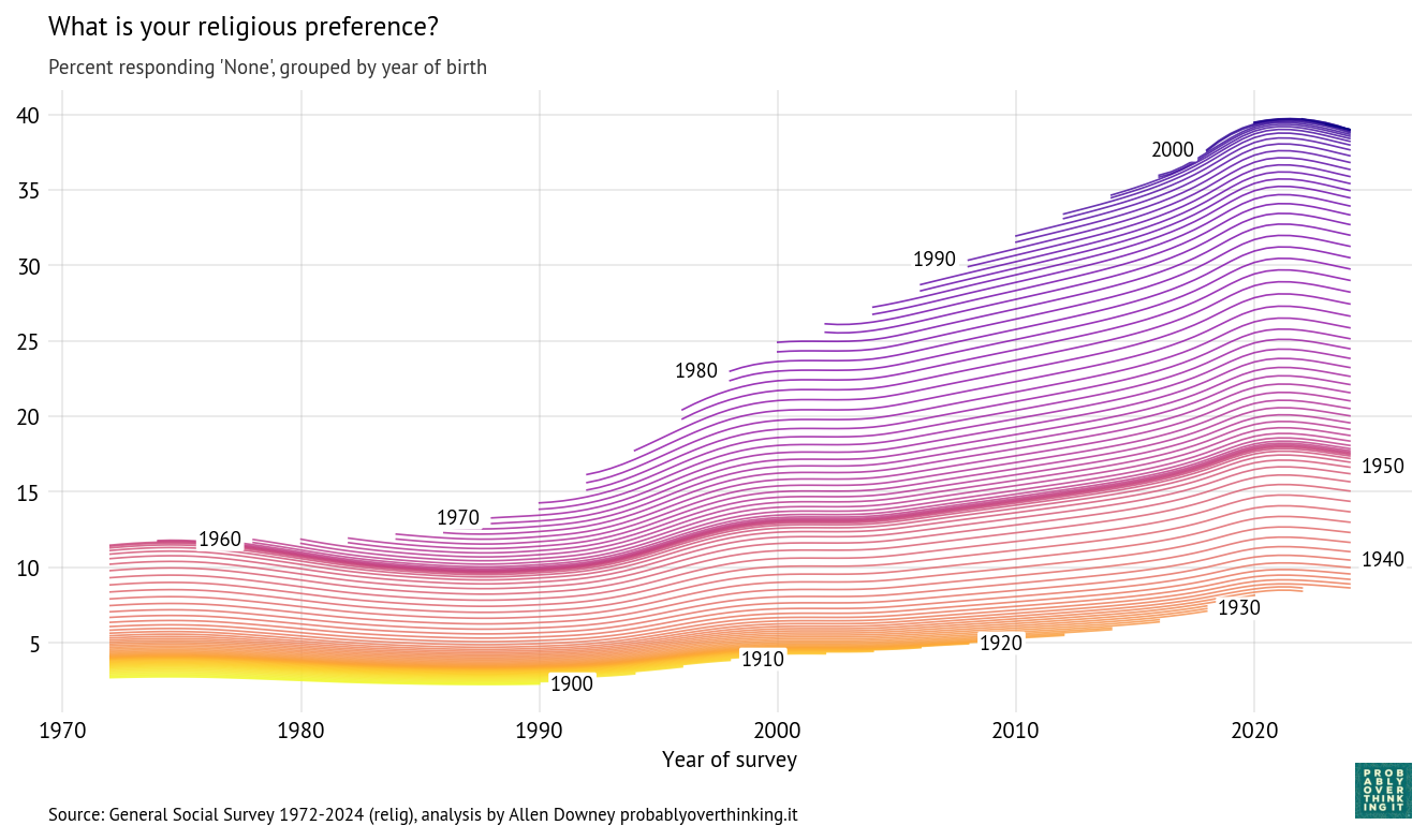
Starting at the bottom, we can see that cohorts born between 1900 and 1930 were not very different — fewer than 10% of them were Nones.

People born in the 1940s were increasingly non-religious, but this first wave of secularization stalled in the cohorts born in the 1950s. The second wave got started with people born in the 1960s, and continued until the 2000s cohorts, where it seems to have stalled again.

Decomposition

With these trajectories, we can decompose the cohort and period effects. The following figure shows the cohort effect, standardized by holding the period effect constant.

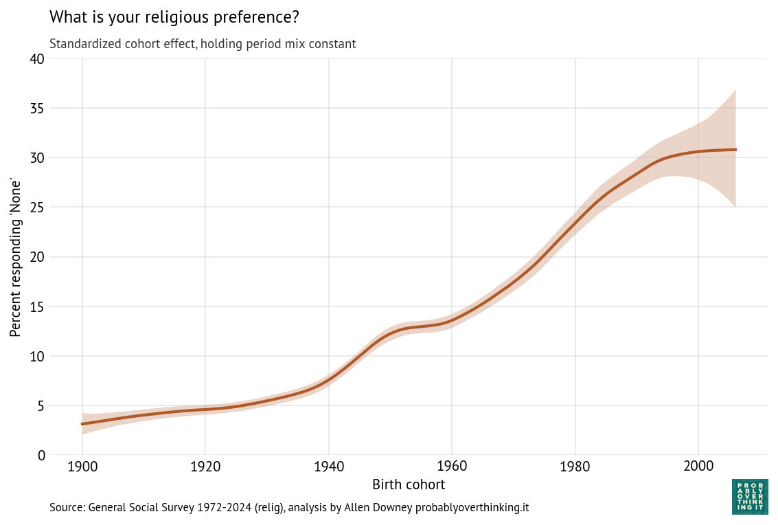
As we saw in the previous figure, there was a period of relatively fast change in the 1940s cohorts that stalled among people born in the 1950s and then resumed among people born in the 1960s through the 1980s (primarily Gen X).

Again, it looks like the most recent cohorts have leveled off, but with the width of the credible interval, it’s possible that the trend has continued or reversed.

The following figure shows the period effect, standardized by holding the cohort mix constant.

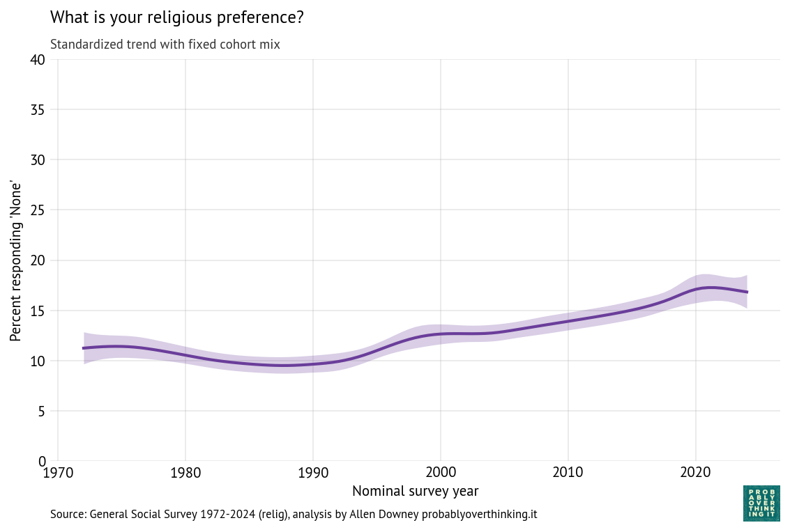
The period effect was generally increasing from 1990 to 2020, but seems to have leveled off or rolled over.

So, if the rise of the Nones has stalled, at least temporarily, it seems to be a combination of a cohort effect among people born after 2000 and a period effect starting around 2020. This decomposition suggests we should look for at least two kinds of explanations:

• Differences in the childhood of people born after 2000 that might make them more likely to have a religious affiliation as young adults, and
• Events since 2020 that have affected all cohorts in ways that might make them more religious.

I’ll hold off on speculating.

For purposes of comparison, here is the trend from the time-only model (blue) and the standardized time trend from the time-cohort model (purple).

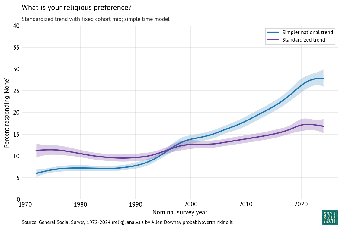
The difference between these lines is the part of the change due to the cohort effect. So we can see that most of the change over this interval is due to generational replacement rather than disaffiliation.

Methods: Details about the model are in the Technical Report.