As people get older, do they become more racist, sexist, and homophobic? To find out, you could use data from the General Social Survey (GSS), which asks questions like:
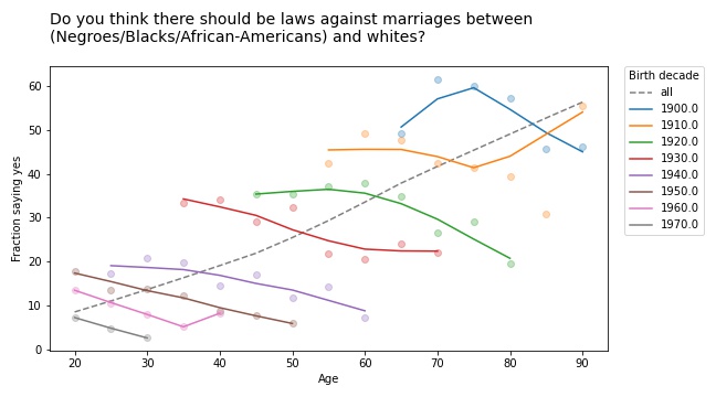
Do you think there should be laws against marriages between Blacks/African-Americans and whites?
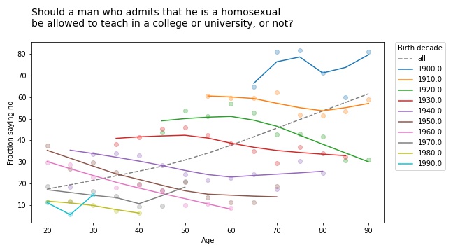
Should a man who admits[mfn]If you find the wording of this question problematic, remember that it was written in 1970 and reflects mainstream views at the time. It persists because, in order to support time series analysis, the GSS generally avoids changing the wording of questions.[/mfn] that he is a homosexual be allowed to teach in a college or university, or not?
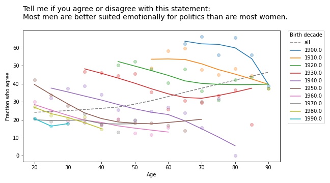
Tell me if you agree or disagree with this statement: Most men are better suited emotionally for politics than are most women.
If you plot the answers to these questions as a function of age, you find that older people are, in fact, more racist, sexist, and homophobic than younger people. But that’s not because they are old; it’s because they were born, raised, and educated during a time when large fractions of the population were racist, sexist homophobes.
In other words, it’s primarily a cohort effect, not an age effect. We can see that if we group respondents by birth cohort and plot their responses by age. Here are the results for the first question:
The circle markers show the proportion of respondents who got this question wrong (no other way to put it); the lines show local regressions through the markers.
The dashed gray line shows the overall trend, if we don’t group by cohort. Sure enough, when this question was asked between 1972 and 2002, older respondents were substantially more likely to support laws against marriage between people of difference races.
But when we group by decade of birth, we see:
A cohort effect: people born later are less racist.
A period effect: within every cohort, people get less racist over time.
The results are similar for the second question:
If you thought the racism was bad, get a load of the homophobia!
But again, all birth cohorts became more tolerant over time (even the people born in the 19-aughts, though it doesn’t look it). And again, there is no age effect; people do not become homophobic as they age.
They don’t get more sexist, either:
Simpson’s Paradox
These are all examples of Simpson’s paradox, where the trend in every group goes in one direction, and the overall trend goes in the other direction. It’s called a paradox because many people find it counterintuitive at first. But once you have seen a few examples, like the ones I wrote about this, this, and this previous article, it gets to be less of a surprise.
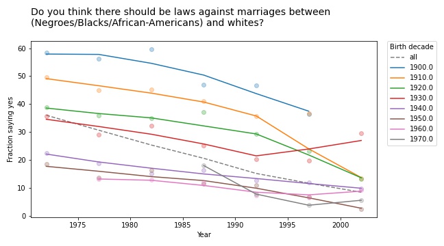
And if you pay attention, it can be a hint that there is something wrong with your model. In this case, it is a symptom that we are looking at the data the wrong way. If we suspect that the changes we see are due to cohort and period, rather than age, we can check by plotting over time, rather than age, like this:
Every cohort is less racist than its predecessor, every cohort gets less racist over time, and the overall trend goes in the same direction, so Simpson’s paradox is resolved.
Or maybe it persists in a weaker form: the overall trend is steeper than the trend in any of the cohorts, because in addition to the cohort effect and the period effect, we also see the effect of generational replacement.
This article is part of a series where I search the GSS for examples of Simpson’s paradox. More coming soon!
Is Simpson’s paradox a mathematical curiosity or something that matters in practice? To answer this question, I’m searching the General Social Survey (GSS) for examples. Last week I published the first batch, examples where we group people by decade of birth and plot their opinions over time. In this article I present the next batch, grouping by education and plotting over time.
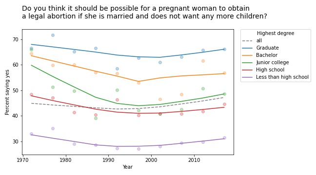
The first example I found is in the responses to this question: “Please tell me whether or not you think it should be possible for a pregnant woman to obtain a legal abortion if she is married and does not want any more children?”
If we group respondents by the highest degree they have earned and compute the fraction who answer “yes” over time, the results meet the criteria for Simpson’s paradox: in every group, the trend over time is downward, but if we put the groups together, the overall trend is upward.
However, if we plot the data, we see that this example is not entirely satisfying.
The markers show the fraction of respondents in each group who answered “yes”; the lines show local regressions through the markers.
In all groups, support for legal abortion (under the specified condition) was decreasing until the 1990s, then started to increase. If we fit a straight line to these curves, the estimated slope is negative. And if we fit a straight line to the overall curve, the estimated slope is positive.
But in both cases, the result doesn’t mean very much because we’re fitting a line to a curve. This is one of many examples I have seen where Simpson’s paradox doesn’t happen because anything interesting is happening in the world; it is just an artifact of a bad model.
This example would have been more interesting in 2002. If we run the same analysis using data from 2002 or earlier, we see a substantial decrease in all groups, and almost no change overall. In that case, the paradox is explained by changes in educational level. Between 1972 and 2002, the fraction of people with a college degree increased substantially. Support for abortion was decreasing in all groups, but more and more people were in the high-support groups.
Free speech
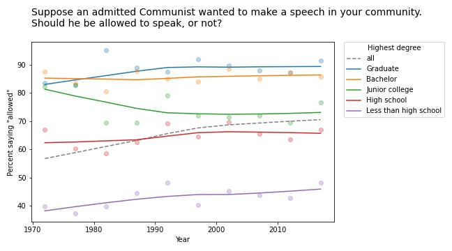
We see a similar pattern in many of the questions related to free speech. For example, the GSS asks, “Suppose an admitted Communist wanted to make a speech in your community. Should he be allowed to speak, or not?” The following figure shows the fraction of respondents at each education level who say “allowed to speak”, plotted over time.
The differences between the groups are big: among people with a bachelor’s or advanced degree, almost 90% would allow an “admitted” Communist to speak; among people without a high school diploma it’s less than 50%. (If you are curious about the wording of questions like this, remember that many GSS questions were written in the 1970s and, for purposes of comparison over time, they avoid changing the text.)
The responses have changed only slightly since 1973: in most groups, support has increased a little; among people with a junior college degree, it has decreased a little.
But overall support has increased substantially, for the same reason as in the previous example: the number of people at higher levels of education increased during this interval.
Whether this is an example of Simpson’s paradox depends on the definition. But it is certainly an example where we see one story if we look at the overall trend and another story if we look at the subgroups.
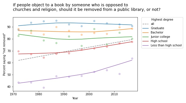
Other questions related to free speech show similar trends. For example, the GSS asks: “There are always some people whose ideas are considered bad or dangerous by other people. For instance, somebody who is against all churches and religion. If some people in your community suggested that a book he wrote against churches and religion should be taken out of your public library, would you favor removing this book, or not?”
The following figure shows the fraction of respondents who say the book should not be removed:
Again, respondents with more education are more likely to support free speech (and probably less hostile to the non-religious, as well). But in this case support is increasing among people with less education. So the overall trend we see is really the sum of two trends: increases within some groups in addition to shifts between groups.
In this example, the overall slope is steeper than the estimated slope in any group. That would be surprising if you expected the overall slope to be like a weighted average of the group slopes. But as all of these examples show, it’s not.
This article presents examples of Simpson’s paradox, and related patterns, when we group people by education level and plot their responses over time. In the next article we’ll see what happens when we groups people by age.
I added a lot of new examples and exercises, most from classes I taught using the first edition.
I rewrote all of the code using NumPy, SciPy, and Pandas (rather than basic Python types). The new code is shorter, clearer, and faster!
For every chapter, there’s a Jupyter notebook where you can read the text, run the code, and work on exercises. You can run the notebooks on your own computer or, if you don’t want to install anything, you can run them on Colab.
More generally, the second edition reflects everything I’ve learned in the 10 years since I started the first edition, and it benefits from the comments, suggestions, and corrections I’ve received from readers. I think it’s really good!
Years ago I told one of my colleagues about my Data Science class and he asked if I taught Simpson’s paradox. I said I didn’t spend much time on it because, I opined, it is a mathematical curiosity unlikely to come up in practice. My colleague was shocked and dismayed because, he said, it comes up all the time in his field (psychology).
And that got me thinking about my old friend, the General Social Survey (GSS). So I’ve started searching the GSS for instances of Simpson’s paradox. I’ll report what I find, and maybe we can get a sense of (1) how often it happens, (2) whether it matters, and (3) what to do about it.
I’ll start with examples where the x-variable is time. For y-variables, I use about 120 questions from the GSS. And for subgroups, I use race, sex, political alignment (liberal-conservative), political party (Democrat-Republican), religion, age, birth cohort, social class, and education level. That’s about 1000 combinations.
Of these, about 10 meet the strict criteria for Simpson’s paradox, where the trend in all subgroups goes in the same direction and the overall trend goes in the other direction. On examination, most of them are not very interesting. In most cases, the actual trend is nonlinear, so the parameters of the linear model don’t mean very much.
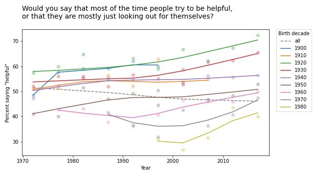
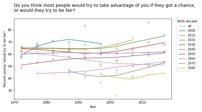
But a few of them turn out to be interesting, at least to me. For example, the following figure shows the fraction of respondents who think “most of the time people try to be helpful”, plotted over time, grouped by decade of birth. The markers show the percentage in each group during each interval; the lines show local regressions.
Within each group, the trend is positive: apparently, people get more optimistic about human nature as they age. But overall the trend is negative. Why? Because of generational replacement. People born before 1940 are substantially more optimistic than people born later; as old optimists die, they are being replaced by young pessimists.
Based on this example, we can go looking for similar patterns in other variables. For example, here are the results from a related question about fairness.
Again, old optimists are being replaced by young pessimists.
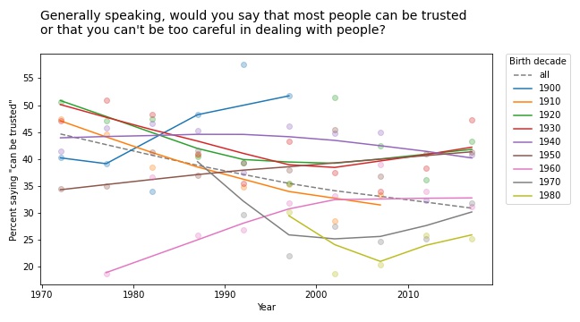
For a similar question about trust, the results are a little more chaotic:
Some groups are going up and others down, so this example doesn’t meet the criteria for Simpson’s paradox. But it shows the same pattern of generational replacement.
Old conservatives, young liberals
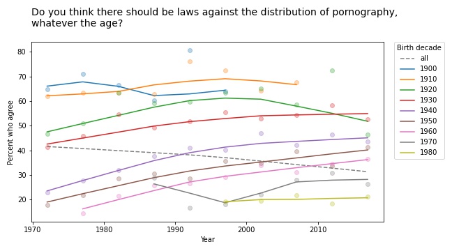
Questions related to prohibition show similar patterns. For example, here are the responses to a question about whether pornography should be illegal.
In almost every group, support for banning pornography has increased over time. But recent generations are substantially more tolerant on this point, so overall support for prohibition is decreasing.
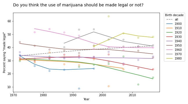
The results for legalizing marijuana are similar.
In most groups, support for legalization has gone down over time; nevertheless, through the power of generational replacement, overall support is increasing.
So far, I think this is more interesting than Derek Jeter’s batting average. More examples coming soon!
Bayesian and frequentist results are not the same, ever
I often hear people say that the results from Bayesian methods are the same as the results from frequentist methods, at least under certain conditions. And sometimes it even comes from people who understand Bayesian methods.
Today I saw this tweet from Julia Rohrer: “Running a Bayesian multi-membership multi-level probit model with a custom function to generate average marginal effects only to find that the estimate is precisely the same as the one generated by linear regression with dummy-coded group membership.” [emphasis mine]
Which elicited what I interpret as good-natured teasing, like this tweet from Daniël Lakens: “I always love it when people realize that the main difference between a frequentist and Bayesian analysis is that for the latter approach you first need to wait 24 hours for the results.”
Ok, that’s funny, but there is a serious point here I want to respond to because both of these comments are based on the premise that we can compare the results from Bayesian and frequentist methods. And that’s not just wrong, it is an important misunderstanding.
You can’t compare results from Bayesian and frequentist methods because the results are different kinds of things. Results from frequentist methods are generally a point estimate, a confidence interval, and/or a p-value. Each of those results is an answer to a different question:
Point estimate: If I have to pick a single value, which one minimizes a particular cost function under a particular set of constraints? For example, which one minimizes mean squared error while being unbiased?
Confidence interval: If my estimated parameters are correct and I run the experiment again, how much would the results vary due to random sampling?
p-value: If my estimated parameters are wrong and the actual effect size is zero, what is the probability I would see an effect as big as the one I saw?
In contrast, the result from Bayesian methods is a posterior distribution, which is a different kind of thing from a point estimate, an interval, or a probability. It doesn’t make any sense to say that a distribution is “the same as” or “close to” a point estimate because there is no meaningful way to compute a distance between those things. It makes as much sense as comparing 1 second and 1 meter.
If you have a posterior distribution and someone asks for a point estimate, you can compute one. In fact, you can compute several, depending on what you want to minimize. And if someone asks for an interval, you can compute one of those, too. In fact, you could compute several, depending on what you want the interval to contain. And if someone really insists, you can compute something like a p-value, too.
But you shouldn’t.
The posterior distribution represents everything you know about the parameters; if you reduce it to a single number, an interval, or a probability, you lose useful information. In fact, you lose exactly the information that makes the posterior distribution useful in the first place.
It’s like comparing a car and an airplane by driving the airplane on the road. You would conclude that the airplane is complicated, expensive, and not particularly good as a car. But that would be a silly conclusion because it’s a silly comparison. The whole point of an airplane is that it can fly.
And the whole point of Bayesian methods is that a posterior distribution is more useful than a point estimate or an interval because you can use it to guide decision-making under uncertainty.
For example, suppose you compare two drugs and you estimate that one is 90% effective and the other is 95% effective. And let’s suppose that difference is statistically significant with p=0.04. For the next patient that comes along, which drug should you prescribe?
You might be tempted to prescribe the second drug, which seems to have higher efficacy. However:
You are not actually sure it has higher efficacy; it’s still possible that the first drug is better. If you always prescribe the second drug, you’ll never know.
Also, point estimates and p-values don’t help much if one of the drugs is more expensive or has more side effects.
With a posterior distribution, you can use a method like Thompson sampling to balance exploration and exploitation, choosing each drug in proportion to the probability that it is the best. And you can make better decisions by maximizing expected benefits, taking into account whatever factors you can model, including things like cost and side effects (which is not to say that it’s easy, but it’s possible).
Bayesian methods answer different questions, provide different kinds of answers, and solve different problems. The results are not the same as frequentist methods, ever.
Conciliatory postscript: If you don’t need a posterior distribution — if you just want a point estimate or an interval — and you conclude that you don’t need Bayesian methods, that’s fine. But it’s not because the results are the same.
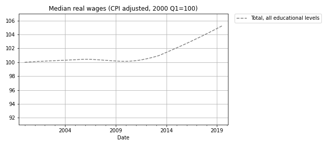
I have good news and bad news. First the good news: after a decade of stagnation, real wages have been rising since 2010. The following figure shows weekly wages for full-time employees (source), which I adjusted for inflation and indexed so the series starts at 100.
Real wages in 2019 Q3 were about 5% higher than in 2010.
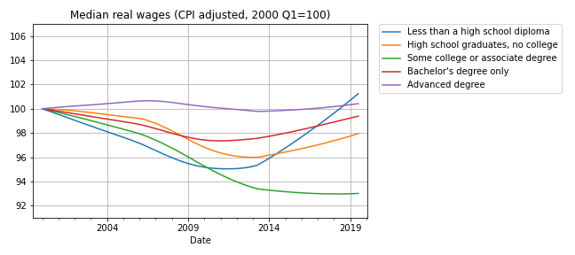
Now here’s the bad news: at every level of education, real wages are lower now than in 2000, or practically the same. The following figure shows real weekly wages grouped by educational attainment:
For people with some college or an associate degree, real wages have fallen by about 5% since 2000 Q1. People with a high school diploma or a bachelor’s degree are making less money, too. People with advanced degrees are making about the same, and high school dropouts are doing slightly better.
But the net change for every group is substantially less than the 5% increase we see if we put the groups together. How is that even possible?
The answer is Simpson’s paradox, which is when a trend appears in every subgroup, but “disappears or reverses when these groups are combined”. In this case, real wages are declining or stagnant in every subgroup, but when we put the groups together, wages are increasing.
In general, Simpson’s paradox can happen when there is a confounding variable that interacts with the variables you are looking at. In this example, the variables we’re looking at are real wages, education level, and time. So here’s my question: what is the confounding variable that explains these seemingly impossible results?
Before you read the next section, give yourself time to think about it.
Credit: I got this example from a 2013 article by Floyd Norris, who was the chief financial correspondent of The New York Times at the time. He responded very helpfully to my request for help replicating his analysis.
The answer
The key (as Norris explained) is that the fraction of people in each educational level has changed. I don’t have the number from the BLS, but we can approximate them with data from the General Social Survey (GSS). It’s not exactly the same because:
The GSS represents the adult residents of the U.S.; the BLS sample includes only people employed full time.
The GSS data includes number of years of school, so I used that to approximate the educational levels in the BLS dataset. For example, I assume that someone with 12 years of school has a high school diploma, someone with 16 years of school has a bachelor’s degree, etc.
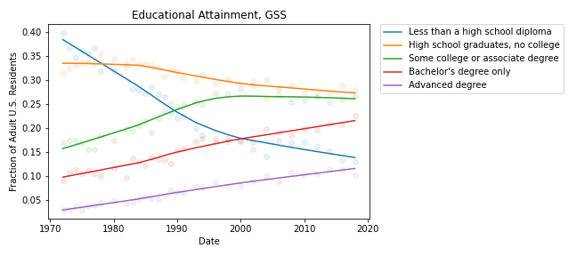
With those caveats, the following figure shows the fraction of GSS respondents in each educational level, from 1973 to 2018:
During the relevant period (from 2000 to 2018), the fraction of people with bachelor’s and advanced degrees increased substantially, and the fraction of high school dropouts declined.
These changes are the primary reason for the increase in median real wages when we put all educational levels together. Here’s one way to think about it:
If you compare two people with the same educational level, one in 2000 and one in 2018, the one in 2018 is probably making less money, in real terms.
But if you compare two people, chosen at random, one in 2000 and one in 2018, the one in 2018 is probably making more money, because the one in 2018 probably has more education.
These changes in educational attainment might explain the paradox, but the explanation raises another question: The same changes were happening between 2000 and 2010, so why were real wages flat during that interval?
I’m not sure I know the answer, but it looks like wages at each level were falling more steeply between 2000 and 2010; after that, some of them started to recover. So maybe the decreases within educational levels were canceled out by the shifts between levels, with a net change close to zero.
And there’s one more question that nags me: Why are real wages increasing for people with less than a high school diploma? With all the news stories about automation and the gig economy, I expected people in this group to see decreasing wages.
The resolution of this puzzle might be yet another statistical pitfall: survivorship bias. The BLS dataset reports median wages for people who are employed full-time. So if people in the bottom half of the wage distribution lose their jobs, or shift to part-time work, the median of the survivors goes up.
And that raises one final question: Are real wages going up or not?
This article is like a pre-excerpt from my forthcoming book, Probably Overthinking It: a revised version of this article make up part of the chapter about Berkson’s paradox. If you would like to get an occasional update about the book, please join my mailing list.
Suppose one day you visit Representative College, where the student body is a representative sample of the college population. You meet a randomly chosen student and you learn (because it comes up in conversation) that they got a 600 on the SAT Verbal test, which is about one standard deviation above the mean. What do you think they got on the SAT Math test?
A: 600 or more
B: Between 500 and 600 (above the mean)
C: Between 400 and 500 (below the mean)
D: 400 or less
If you chose B, you are right! Scores on the SAT Math and Verbal tests are correlated, so if someone is above average on one, they are probably above average on the other. The correlation coefficient is about 0.7, so people who get 600 on the verbal test get about 570 on the math test, on average.
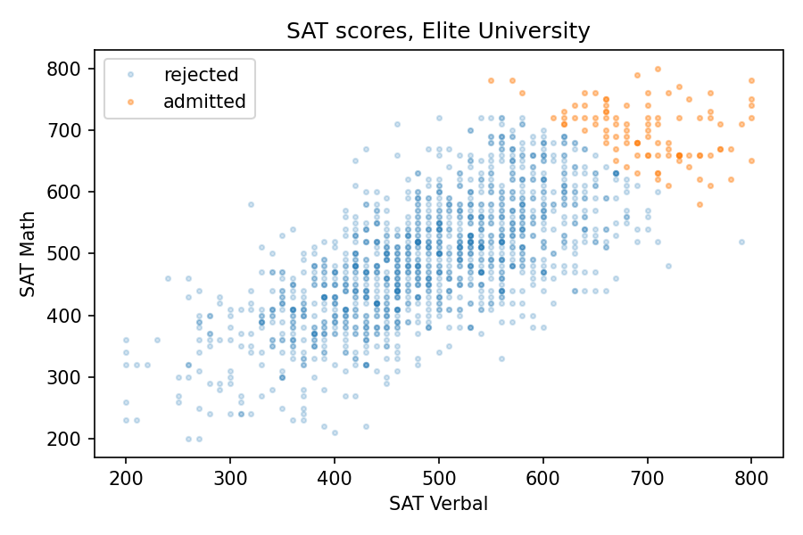
Now suppose you visit Elite University, where the average score on both tests is 700. You meet a randomly chosen student and you learn (because they bring it up) that they got a 750 on the verbal test, which is about one standard deviation above the mean at E.U. What do you think they got on the math test?
A: 750 or more
B: Between 700 and 750 (above the mean)
C: Between 650 and 700 (below the mean)
D: 650 or less
If you chose B again, you are wrong! Among students at E.U., the correlation between test scores is negative. If someone is above average on one, they are probably below average on the other.
This is an example of Berkson’s paradox, which is a form of selection bias. In this case, the selection is the college admission process, which is partly based on exam scores. And the effect, at elite colleges and universities, is a negative correlation between test scores, even though the correlation in the general population is positive.
Data
To see how it works in this example, let’s look at some numbers. I got data from the National Longitudinal Survey of Youth 1997 (NLSY97), which “follows the lives of a sample of [8,984] American youth born between 1980-84”. The public data set includes the participants’ scores on several standardized tests, including the SAT and ACT.
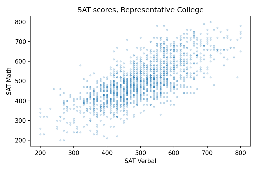
About 1400 respondents took the SAT. Their average and standard deviation are close to the national average (500) and standard deviation (100). And the correlation is about 0.73. To get a sense of how strong that is, here’s what the scatter plot looks like.
Since the correlation is about 0.7, someone who is one standard deviation above the mean on the verbal test is about 0.7 standard deviations above the mean on the math test, on average. So at Representative College, if we select people with verbal scores near 600, their average math score is about 570.
Elite University
Now let’s see what happens when we select students for Elite University. Suppose that in order to get into E.U., your total SAT score has to be 1320 or higher. If we select students who meet or exceed that threshold, their average on both tests is about 700, and the standard deviation is about 50.
Among these students, the correlation between test scores is about -0.33, which means that if you are one standard deviation above the E.U. mean on one test, you are about 0.33 standard deviations below the E.U. mean on the other, on average.
The following figure shows why this happens:
The students who meet the admission requirements at Elite University form a triangle in the upper right, with a moderate negative correlation between test scores.
Specialized University
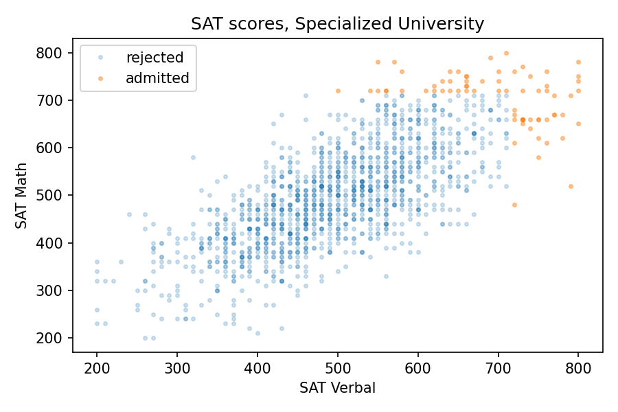
Of course, most admissions decisions are based on more than the sum of two SAT scores. But we get the same effect even if the details of the admission criteria are different. For example, suppose another school, Specialized University, admits students if either test score is 720 or better, regardless of the other score.
With this threshold, the mean for both tests is close to 700, the same as Elite University, and the standard deviations are a little higher. But again, the correlation is negative, and a little stronger than at E.U., about -0.38, compared to -0.33.
The following figure shows the distribution of scores for admitted students.
There are three kinds of students Specialized University: good at math, good at language, and good at both. But the first two groups are bigger than the third, so the overall correlation is negative.
Sweep the Threshold
Now let’s see what happens as we vary the admissions requirements. I’ll go back to the previous version, where admission depends on the total of the two tests, and vary the threshold.
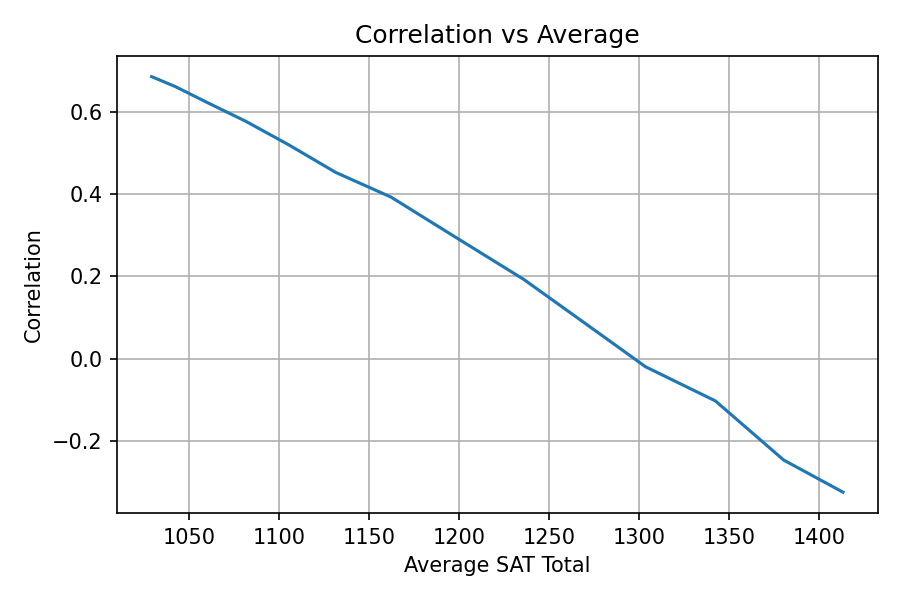
As we increase the threshold, the average total score increases and the correlation decreases. The following figure shows the results.
At Representative College, where the average total SAT is near 1000, test scores are strongly correlated. At Elite University, where the average is over 1400, the correlation is moderately negative.
Secondtier College
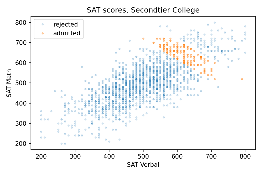
But at a college that is selective but not elite, the effect might be even stronger than that. Suppose at Secondtier College (it’s pronounced “seh con’ tee ay'”), a student with a total score of 1220 or more is admitted, but a student with 1320 or more is likely to go somewhere else.
In that case, the average total score would be about 1260. So, based on the parameter sweep in the previous section, we would expect a weak positive correlation, but the correlation is actually strongly negative, about -0.8! The following picture shows why.
At Secondtier, if you meet a student who got a 690 on the math test, about one standard deviation above the mean, you should expect them to get a 580 on the verbal test, on average. That’s a remarkable effect.
Summary
Among the students at a given college or university, verbal skills and math skills might be strongly correlated, anti-correlated, or uncorrelated, depending on how the students are selected. This is an example of Berkson’s paradox.
If you enjoy this kind of veridical paradox, you might like my previous article “The Inspection Paradox Is Everywhere“. And if you like thinking about probability, you might like the second edition of Think Bayes (affiliate link), which will be published by O’Reilly Media later this month.
Finally, if you have access to standardized test scores at a college or university, and you are willing to compute a few statistics, I would love to compare my results with some real-world data. For students who enrolled, I would need
Mean and standard deviation for each section of the SAT or ACT.
Correlations between the sections.
The results, if you share them, would appear as a dot on a graph, either labeled or unlabeled at your discretion.
Related:The SAT Math Gap, a Bayesian model of how much of the gender gap in SAT math scores comes from who takes the test (PyData Boston 2025).
A few years ago I wrote an article for the Scientific American blog where I used data from the General Social Survey (GSS) to describe changes in religious affiliation in the U.S.
And in this longer article I described changes in religious belief as well, including belief in God, interpretation of the Bible, and confidence in religious institutions.
Those articles were based on GSS data released in 2017, which included interviews up to 2016. Now the GSS has released additional data from interviews conducted in 2017 and 2018, including young adults born in 1999 and 2000.
So it’s time to update the results.
Religious affiliation by cohort
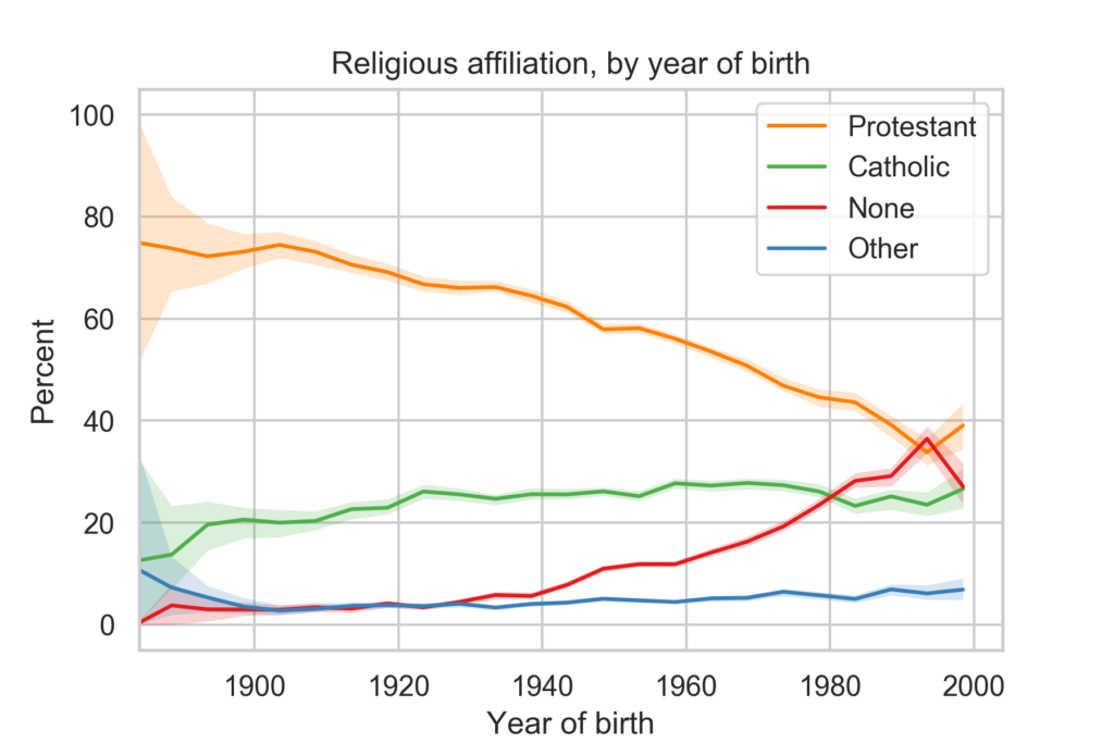
The following figure shows religious affiliation by year of birth.
The youngest group in the survey, people born between 1996 and 2000, depart from several long-term trends:
They are more likely to identify as Protestant than the previous cohort, and slightly more likely to identify as Catholic.
And they are less likely to report no religious preference.
There are only 201 people in this group, so these results might be an anomaly. Data from other sources indicates that young adults are less religious than older groups.
Religious affiliation by year
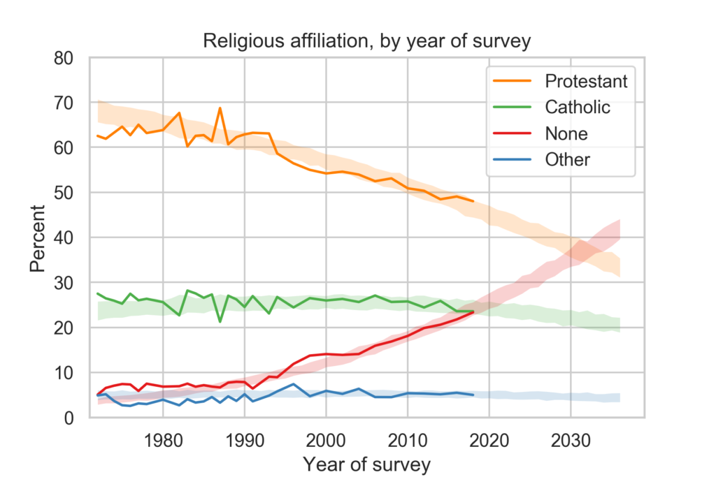
The following figure shows religious affiliation by year of interview along with predictions based on a simple model of generational replacement.
Despite the reversal of trends in the previous figure, the long-term trends in religious affiliation continue:
The fraction of people who identify as Protestant or Christian is declining and accelerating.
The fraction who identify as Catholic has started to decline.
The fraction with no religious affiliation is increasing and accelerating.
Based on the previous batch of data, I predicted that there would be more Nones than Catholics in 2020. With the most recent data, it looks like the cross-over might be ahead of schedule.
On these trends, there will be more Nones than Protestants sometime after 2030.
In the next article, I’ll present related trends in religious belief and confidence in religious institutions.
This topic is part of my book in progress, You Would Choose Now, which uses decades of survey data to track changing attitudes in the United States. The early access edition is available now.
In the last 30 years, college students have become much less religious. The fraction who say they have no religious affiliation has more than tripled, from about 10% to 34%. And the fraction who say they have attended a religious service in the last year fell from more than 85% to 66%.
I’ve been following this trend for a while, using data from the CIRP Freshman Survey, which has surveyed a large sample of entering college students since 1966.
The most recently published data is from “95,505 first-time, full-time freshmen entering 148 baccalaureate institutions” in Fall 2019.
Of course, college students are not a representative sample of the U.S. population. Furthermore, as rates of college attendance have increased, they represent a different slice of the population over time. Nevertheless, surveying young adults over a long interval provides an early view of trends in the general population.
Religious preference
Among other questions, the Freshman Survey asks students to select their “current religious preference” from a list of seventeen common religions, “Other religion,” “Atheist”, “Agnostic”, or “None.”
The options “Atheist” and “Agnostic” were added in 2015. For consistency over time, I compare the “Nones” from previous years with the sum of “None”, “Atheist” and “Agnostic” since 2015.
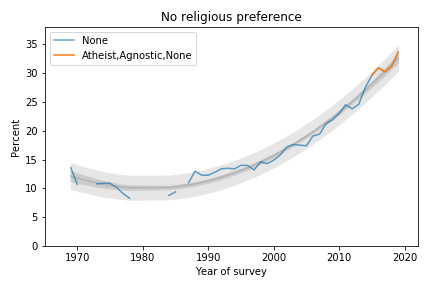
The following figure shows the fraction of Nones from 1969, when the question was added, to 2019, the most recent data available.
Percentage of students with no religious preference from 1969 to 2019.
The blue line shows data until 2015; the orange line shows data from 2015 through 2019. The gray line shows a quadratic fit. The light gray region shows a 95% predictive interval.
The quadratic model continues to fit the data well and the most recent data point is above the trend line, which suggests that the “rise of the Nones” is still accelerating.
Attendance
The survey also asks students how often they “attended a religious service” in the last year. The choices are “Frequently,” “Occasionally,” and “Not at all.” Respondents are instructed to select “Occasionally” if they attended one or more times, so a wedding or a funeral would do it.
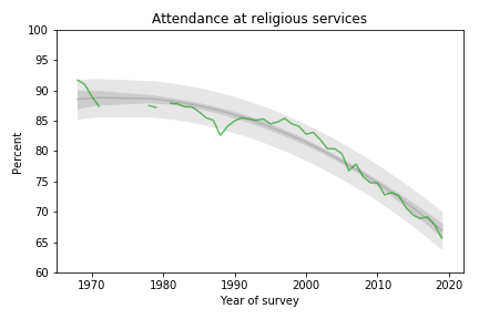
The following figure shows the fraction of students who reported any religious attendance in the last year, starting in 1968. I discarded a data point from 1966 that seems unlikely to be correct.
Percentage of students who reported attending a religious service in the previous year.
About 66% of incoming college students said they attended a religious service in the last year, an all-time low in the history of the survey, and down more than 20 percentage points from the peak.
This curve is on trend, with no sign of slowing down.
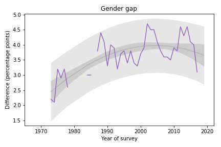
Gender Gap
Female students are more religious than male students. The following graph shows the gender gap over time, that is, the difference in percentages of male and female students with no religious affiliation.
Difference in religious affiliation between male and female students.
The gender gap was growing until recently. It has shrunk in the last 3-4 years, but since it varies substantially from year to year, it is hard to rule out random variation.
Data Source
The American Freshman: National Norms Fall 2019 Stolzenberg, Aragon, Romo, Couch, McLennon, Eagan, and Kang, Higher Education Research Institute, UCLA, June 2020
This topic is part of my book in progress, You Would Choose Now, which uses decades of survey data to track changing attitudes in the United States. The early access edition is available now.
A unique feature of the game is the dice, which yield three possible outcomes, 0, 1, or 2, with equal probability. When you add them up, you get some unusual probability distributions.
There are two phases of the game: During the first phase, players explore a haunted house, drawing cards and collecting items they will need during the second phase, called “The Haunt”, which is when the players battle monsters and (usually) each other.
So when does the haunt begin? It depends on the dice. Each time a player draws an “omen” card, they have to make a “haunt roll”: they roll six dice and add them up; if the total is less than the number of omen cards that have been drawn, the haunt begins.
For example, suppose four omen cards have been drawn. A player draws a fifth omen card and then rolls six dice. If the total is less than 5, the haunt begins. Otherwise the first phase continues.
Last time I played this game, I was thinking about the probabilities involved in this process. For example:
What is the probability of starting the haunt after the first omen card?
What is the probability of drawing at least 4 omen cards before the haunt?
What is the average number of omen cards before the haunt?